Creating Hodograph Plots
This tutorial creates SounderPy Hodograph plots!
Here we will explore:
Building hodographs
Plots in dark mode
Storm relative hodographs
Saving hodograph plots to a file
[1]:
# First lets import SounderPy. Its fun to import as 'spy'!
import sounderpy as spy
Load some data to plot
Here we can load some data with SounderPy.
Let’s investigate DTX (White Lake, MI) observations for a June tornado outbreak in 2015. We can use the get_obs_data() function to do this
[2]:
clean_data = spy.get_obs_data('dtx', '2015', '06', '23', '00')
> OBSERVED DATA ACCESS FUNCTION
  -----------------------------------
    > PROFILE FOUND: DTX on 06/23/2015 at 00z | From UW (ID: 72632)
    > COMPLETE --------
    > RUNTIME: 00:00:06
    > SUMMARY: 00Z Launch for KDTX, White Lake at 06-23-2015-00Z

    > THERMODYNAMICS ---------------------------------------------
    --- SBCAPE: 3040.2 | MUCAPE: 3040.2 | MLCAPE: 2314.7 | MUECAPE: 2846.4
    --- MU 0-3: 99.9 | MU 0-6: 845.9 | SB 0-3: 99.9 | SB 0-6: 845.9

    > KINEMATICS -------------------------------------------------
    --- 0-500 SRW: 43.3 knot | 0-500 SWV: 0.032 | 0-500 SHEAR: 28.8 | 0-500 SRH: 308.5
    --- 1-3km SRW: 33.1 knot | 1-3km SWV: 0.013 | 1-3km SHEAR: 57.3 | | 1-3km SRH: 337.1
    ==============================================================
Build a full hodograph plot
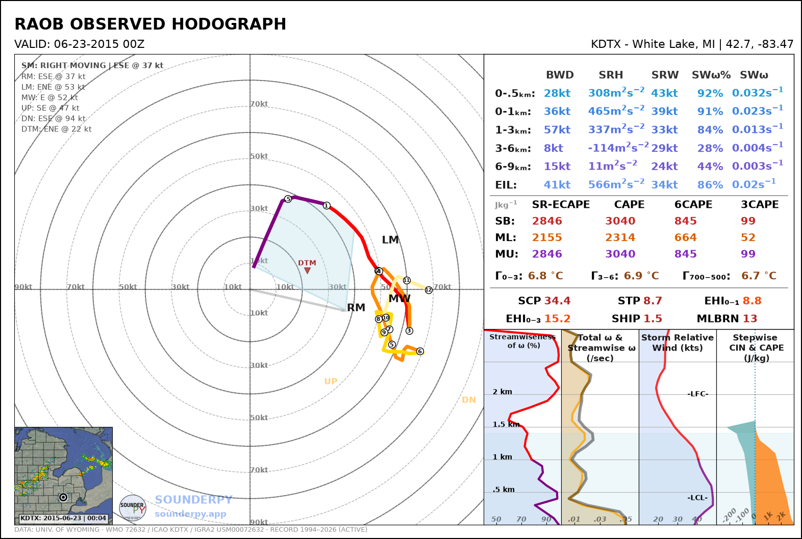
Here we use the most basic version of the build_hodograph() function.
[3]:
# light-mode hodograph
# radar='single' shows the nearest NEXRAD site's reflectivity on the map.
# The default radar mosaic only keeps about the last month, so it can't cover this date.
spy.build_hodograph(clean_data, radar='single')
> HODOGRAPH PLOTTER FUNCTION --
-------------------------------
    > PREPARING DATA
    > BUILDING HODOGRAPH
    > BUILDING MAP INSET
    > RADAR SCAN FOUND: Site: KDTX Scan: 2015-06-23 | 00:04z
Ignoring fixed x limits to fulfill fixed data aspect with adjustable data limits.
    > BUILDING ACCESSORY PLOTS
    > PLOTTING PARAMETERS
    > FIGURE LOADING...
    > COMPLETE --------
    > RUNTIME: 00:00:13
Playing with hodograph settings
The plot above requried a very simple line of code.
Now we can adjust a few settings to customize the plot a little bit.
To do so, let’s first study the build_hodograph() function…
build_hodograph(clean_data, dark_mode=False, storm_motion='right_moving', sr_hodo=False, modify_sfc=None, radar='mosaic', radar_time='sounding', map_zoom=2, hodo_boundary=None, dpi=100, save=False, filename='sounderpy_hodograph', max_levels=250, theme=None)
where:
clean_data(dict, required) – the dictionary of data to be plotteddark_mode(bool, optional, default is False) – True will invert the color scheme for a ‘dark-mode’ hodograph.storm_motion(str or list of floats, optional, default is ‘right_moving’) – the storm motion used for plotting and calculations. Custom storm motions are accepted as a list of floats representing direction and speed. Ex: [270.0, 25.0] where ‘270.0’ is the direction in degrees and ‘25.0’ is the speed in kts. See the documentation for more details.sr_hodo(bool, optional, default is False) – transform the hodograph from ground relative to storm relativemodify_sfc(None or dict, optional, default is None) – adictin the format{'T': 25, 'Td': 21, 'ws': 20, 'wd': 270}to modify the surface values of theclean_datadict. See the documentation for more details.radar(str or None, optional, default is ‘mosaic’) – the radar shown on the map inset: ‘mosaic’, ‘single’ (the nearest NEXRAD site), or None. Note: radar mosaic data only goes back about 1 month from the current date, so use ‘single’ for older cases.radar_time(str or datetime, optional, default is ‘sounding’) – radar valid time: ‘sounding’, ‘now’, or adatetime.map_zoom(int, optional, default is 2) – a ‘zoom’ level for the map inset. Note: setting ``map_zoom=0`` will hide the maphodo_boundary(dict, optional) – draw one or more ‘boundary’ lines on the hodograph, given as angles and colors.dpi(int, optional, default is 100) – resolution of the figure.save(bool, optional, default is False) – whether to show the plot inline or save to a file.filename(str, optional, default is ‘sounderpy_hodograph’) – the filename to save to ifsave=True.max_levels(int or None, optional, default is 250) – the most vertical levels used; longer profiles are thinned. None uses every level.theme(dict, optional) – changes to the figure’s colors, such as{'border': 'k'}.
See every option in detail: https://kylejgillett.github.io/sounderpy/reference/plottingdata.html#building-hodographs
This case is from 2015, older than the radar mosaic archive, so the examples below use radar='single' to show reflectivity from the nearest NEXRAD site.
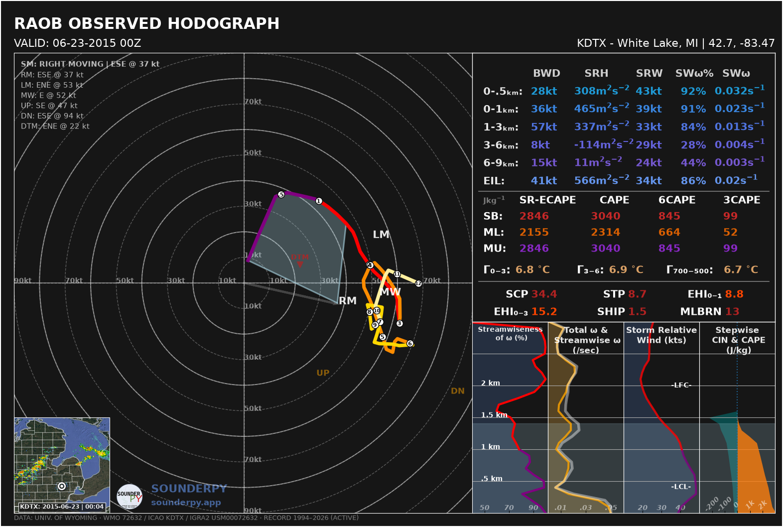
Lets try the dark_mode setting:
[4]:
# dark_mode turned on!
spy.build_hodograph(clean_data, dark_mode=True, radar='single')
> HODOGRAPH PLOTTER FUNCTION --
-------------------------------
    > PREPARING DATA
    > BUILDING HODOGRAPH
    > BUILDING MAP INSET
Ignoring fixed x limits to fulfill fixed data aspect with adjustable data limits.
    > RADAR SCAN FOUND: Site: KDTX Scan: 2015-06-23 | 00:04z
    > BUILDING ACCESSORY PLOTS
    > PLOTTING PARAMETERS
    > FIGURE LOADING...
    > COMPLETE --------
    > RUNTIME: 00:00:04
Storm relative hodographs
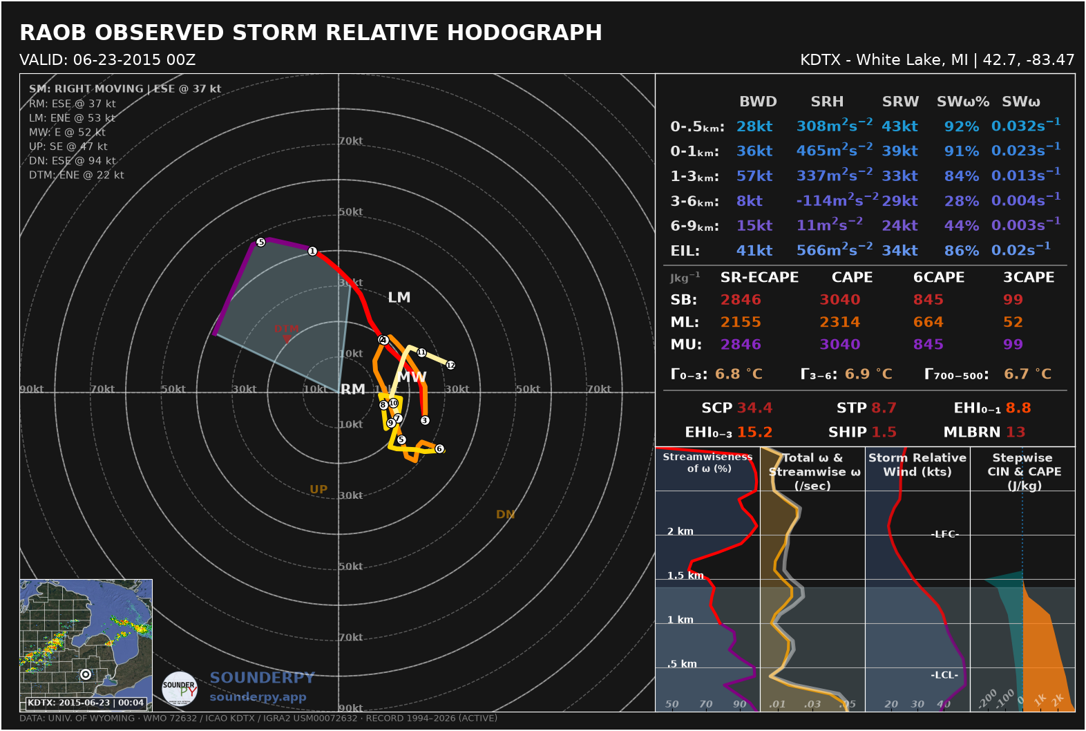
A storm-relative hodograph is a hodograph centered on the storm-motion. In this way we can think more about what the “storm feels”.
A storm-relative hodograph “normalizes all of the seemingly-infinite hodograph shapes into what the supercell actually experiences” - Cameron J Nixon (read more here: https://cameronjnixon.wordpress.com/research/hodographs/)
To create a SounderPy storm relative hodograph, simply use the sr_hodo kwarg, set it equl to True.
NOTE
This will only work if a storm motion exists.
The storm motion defaults to Bunkers Right Moving, but this can be changed with the
storm_motionkwarg.A vertical profile must be over 6km tall for the Bunkers calculation to work, so profiles below this height will still be ‘ground-relative’
[5]:
# storm-relative hodograph!
spy.build_hodograph(clean_data, dark_mode=True, sr_hodo=True, radar='single')
> HODOGRAPH PLOTTER FUNCTION --
-------------------------------
    > PREPARING DATA
    > BUILDING HODOGRAPH
    > BUILDING MAP INSET
    > RADAR SCAN FOUND: Site: KDTX Scan: 2015-06-23 | 00:04z
Ignoring fixed x limits to fulfill fixed data aspect with adjustable data limits.
    > BUILDING ACCESSORY PLOTS
    > PLOTTING PARAMETERS
    > FIGURE LOADING...
    > COMPLETE --------
    > RUNTIME: 00:00:03
Saving plots as a file
By default, SounderPy is set to show plots inline. If you want/need to save them to a file, SounderPy offers that option!
Just set the save kwarg to True, and give it a file name using the filename kwarg!
IMPORTANT NOTE!!!
If your plots come out with a funky layout when displaying them inline, it may be due to your screen resolution.
In the event that this is the case, simply use the
save=Trueoption to save plots to a file!
[6]:
#spy.build_hodograph(clean_data, save=True, filename='sounderpy_2015062300z_DTX')
[ ]: