
Plotting Soundings From Custom Data Sources
Have data that you want to plot on SounderPy plots, but it’s not native to SounderPy? Here’s a way to do so!
This notebook will provide some instructions for getting custom data sources into SounderPy-friendly formats so you can use your data on SounderPy plots.
First, please be sure to read up on SounderPy documentation, specifically the section “What does the data look like?”. Here you can find specific details about the data structure (using a Python dict) that SounderPy plots ingest.
Check it Out: https://kylejgillett.github.io/sounderpy/reference/clean_data_scheme.html
First, let’s investigate SounderPy plot functions, such as build_sounding():
spy.build_sounding(clean_data, save=False, filename='sounderpy_sounding', color_blind=True, dark_mode=False)SounderPy plots need a variable called
clean_data. This is a Python dictionary of vertical profile data and profile metadata.This
dicthas three main sections: the actual profile data, the metadata of the profile’s location (site_info), and the figure titles (titles).You’ll need to create one of these dictionaries out of your data, following the same structure.
The profile data this
dictcontains…clean_data['p']: anarrayof pressure dataclean_data['z']: anarrayof height dataclean_data['T']: anarrayof temperature dataclean_data['Td']: anarrayof dewpoint dataclean_data['u']: anarrayof u-component of wind dataclean_data['v']: anarrayof v-component of wind data
The profile metadata this
dictcontains (viaclean_data['site_info'])…clean_data['site_info']['site-name']a
strrepresenting the name of a profile site, if available (e.g. ‘DTX’)
clean_data['site_info']['site-lctn']a
strrepresenting additional site location information (e.g. ‘MI US’)
clean_data['site_info']['site-latlon']a latitude-longitude pair of
floatsin alist
clean_data['site_info']['site-elv']elevation of the profile
clean_data['site_info']['source']a
strrepresenting the data source name (e.g. ‘RAOB OBSERVED PROFILE’)other sources are… ‘ACARS OBSERVED AIRCRAFT PROFILE’, ‘BUFKIT FORECAST PROFILE’, ‘MODEL REANALYSIS PROFILE’, ‘RAOB OBSERVED PROFILE’
clean_data['site_info']['model']a
strrepresenting the model name, if available (e.g., ‘no-model’ or ‘hrrr’)
clean_data['site_info']['fcst-hour']if a model is used, the forecast hour of the model run as a
str(e.g. ‘no-fcst-hour’ or ‘F01’)
clean_data['site_info']['run-time']if a model is used, the model run time as a
listofstrs
clean_data['site_info']['valid-time']the data’s valid time as a
listofstrs
The figure titles this
dictcontains (viaclean_data['titles'])…clean_data['titles']['top_title']the large title across the top of the figure (e.g. ‘RAOB OBSERVED VERTICAL PROFILE’)
clean_data['titles']['left_title']the smaller title on the left, usually the valid time (e.g. ‘VALID: 05-20-2022 18Z’)
clean_data['titles']['right_title']the smaller title on the right, usually the site and location (e.g. ‘KAPX - GAYLORD, MI | 44.92, -84.72’)
Below is an example:
{'p': array([944. , 926.4, 925. , 894.5, 863.5, 850. , 848. , 833.4, 804.1,
        795. , 775.7, 774. , 748. , 721.2, 720. , 700. , 685. , 674. ,
        670. , 651. , 645.1, 630. , 621.3, 621. , 598.2, 591. , 587. ,
        583. , 572. , 554. , 509. , 500. , 473.6, 471. , 446. , 442. ,
        425. , 418. , 402. , 400. , 399. , 395. , 386. , 382. , 370. ,
        354.7, 354. , 336. , 311.2, 300. , 297. , 279. , 250. , 241. ,
        239. , 237.6, 232. , 200. , 194. , 190. , 188. , 170. , 168.9,
        165. , 162. , 161. , 160.6, 155. , 152.8, 150. , 138.2, 135. ,
        131.3, 131. , 130. , 127. , 125. , 124.8, 122. , 118.7, 118. ,
        113. , 112. , 111. , 108. , 103. , 102. , 101. , 100. ]) <Unit('hectopascal')>,
 'z': array([  446,   610,   623,   914,  1219,  1356,  1376,  1524,  1829,
         1926,  2134,  2152,  2438,  2743,  2757,  2990,  3168,  3300,
         3349,  3584,  3658,  3850,  3962,  3966,  4267,  4364,  4419,
         4473,  4625,  4877,  5542,  5680,  6096,  6137,  6550,  6617,
         6911,  7035,  7323,  7360,  7378,  7452,  7620,  7696,  7925,
         8230,  8243,  8612,  9144,  9400,  9470,  9900, 10640, 10880,
        10935, 10973, 11128, 12070, 12260, 12389, 12454, 13067, 13106,
        13246, 13356, 13394, 13411, 13628, 13716, 13830, 14326, 14466,
        14630, 14645, 14690, 14831, 14927, 14935, 15075, 15240, 15278,
        15544, 15599, 15655, 15826, 16123, 16184, 16247, 16310]) <Unit('meter')>,
 'T': array([ 26. ,  24.3,  24.2,  21.7,  19.2,  18. ,  17.4,  16.4,  14.3,
         13.6,  13.4,  13.4,  10.9,   8.3,   8.2,   6.4,   5.2,   5.8,
          6. ,   4.2,   3.6,   2. ,   2.4,   2.4,   0.2,  -0.5,  -0.7,
         -0.5,  -0.9,  -3.1,  -9.1, -10.3, -14.1, -14.5, -16.9, -16.7,
        -19.1, -19.7, -22.3, -22.5, -22.5, -22.5, -23.9, -24.5, -26.7,
        -29.6, -29.7, -32.7, -36.1, -37.7, -37.9, -41.1, -47.1, -49.3,
        -49.5, -49.8, -51.1, -59.3, -61.3, -62.3, -62.9, -68.1, -68.3,
        -68.9, -68.3, -63.9, -63.8, -62.1, -62.8, -63.7, -68.5, -69.9,
        -70.3, -70.3, -68.1, -66.5, -65.3, -65.3, -65.3, -63.8, -63.5,
        -62.9, -61.9, -60.5, -59.1, -58.7, -57.5, -55.3, -55.3]) <Unit('degree_Celsius')>,
 'Td': array([ 17. ,  16.3,  16.2,  15.6,  15. ,  14.7,  14.8,  14.2,  13. ,
         12.6,  10. ,   9.8,   8.7,   7.5,   7.4,   5.3,   4.1,  -1.2,
         -3. ,  -3.8,  -3.6,  -3. ,  -4.5,  -4.6,  -4.4,  -4.3,  -5.3,
         -8.5, -12.9, -14.1, -17.1, -17.3, -17.4, -17.4, -20.1, -22.7,
        -26.1, -29.7, -31.3, -31.5, -31.5, -35.5, -37.6, -38.5, -36.8,
        -34.5, -34.4, -36.4, -39.8, -41.4, -41.5, -45.7, -50.8, -53. ,
        -54.3, -54.7, -56.1, -64.3, -66.3, -67.3, -66.9, -72. , -72.2,
        -72.9, -72.5, -68.5, -68.4, -67.1, -67.8, -68.7, -73.5, -74.9,
        -75.3, -75.3, -74.1, -74.5, -74.3, -74.4, -76.3, -76.5, -76.5,
        -78.9, -78.9, -78.5, -79.1, -83.7, -83.5, -83.3, -83.3]) <Unit('degree_Celsius')>,
 'u': array([ 10.7246222 ,  10.60660172,  10.60660172,  17.        ,
         22.36948102,  26.99707961,  26.99707961,  27.63986722,
         31.81980515,  34.37362398,  39.83431104,  39.83431104,
         42.13244437,  45.05336244,  45.05336244,  39.83431104,
         39.99960775,  40.12982058,  40.22445359,  40.28302882,
         40.30508653,  40.30508653,  40.30508653,  40.30508653,
         55.92124435,  56.73165519,  56.73165519,  57.52478501,
         57.50175672,  58.97894719,  60.00171105,  60.62177826,
         64.08587988,  64.08587988,  58.51531863,  58.51531863,
         55.35225748,  53.05840464,  49.9682747 ,  49.9682747 ,
         49.9682747 ,  48.32997061,  44.23421039,  43.93899135,
         44.16729559,  50.78742675,  50.78742675,  50.78742675,
         51.60657879,  51.09549882,  51.09549882,  53.85980316,
         57.09739058,  55.28477501,  54.37846722,  54.37846722,
         55.28477501,  61.62892952,  64.34785288,  67.06677624,
         67.97308403,  77.94246969,  78.84877747,  91.15018422,
         99.6074178 , 102.42649567, 102.42649567,  80.39200027,
         71.59831518,  69.53725394,  67.61480784,  52.13005469,
         33.7059555 ,  34.47199994,  37.03650542,  45.28821067,
         51.09549882,  51.09549882,  45.033321  ,  37.23909236,
         37.60864741,  37.74069899,  38.27679749,  37.58770483,
         37.48920614,  36.5444686 ,  36.63991854,  35.80278823,
         35.86300913]) <Unit('knot')>,
 'v': array([ 8.99902654, 10.60660172, 10.60660172, 29.44486373, 31.94692973,
        32.17386661, 32.17386661, 32.93991105, 31.81980515, 32.05392292,
        33.4249557 , 33.4249557 , 35.35331853, 31.546704  , 31.546704  ,
        33.4249557 , 34.77112854, 36.13305274, 37.5099098 , 38.90086875,
        40.30508653, 40.30508653, 40.30508653, 40.30508653, 46.92349551,
        45.94038855, 45.94038855, 44.9432877 , 43.33068167, 41.29750342,
        36.05266524, 35.        , 37.        , 37.        , 36.56442923,
        36.56442923, 35.94617631, 35.78834582, 34.98816262, 34.98816262,
        34.98816262, 33.84100974, 30.97312756, 29.63722388, 25.5       ,
        35.56173905, 35.56173905, 35.56173905, 36.13531549, 29.5       ,
        29.5       , 28.63776533, 26.62495049, 25.77971397, 25.3570957 ,
        25.3570957 , 25.77971397, 28.7380418 , 30.00589658, 31.27375137,
        31.69636963, 36.34517051, 36.76778877, 33.1759539 , 36.25413519,
        37.28019562, 37.28019562, 35.79282459, 33.38684268, 25.30949061,
        18.11733316, 25.42552651, 28.28265483, 28.92544244, 28.93608934,
        29.41050789, 29.5       , 29.5       , 26.        , 21.5       ,
        20.84681367, 16.01997627, 14.69308593, 13.68080573, 10.74985688,
         5.78807521,  5.14940474,  3.76302468,  3.13760674]) <Unit('knot')>,
 'site_info': {'site-id': 'KAPX',
  'site-name': 'GAYLORD',
  'site-lctn': 'MI US',
  'site-latlon': [44.92, -84.72],
  'site-elv': 446.0,
  'source': 'RAOB OBSERVED PROFILE',
  'model': 'no-model',
  'fcst-hour': 'no-fcst-hour',
  'run-time': ['no-run-time'],
  'valid-time': ['2022', '05', '20', '18']},
 'titles': {'top_title': 'RAOB OBSERVED VERTICAL PROFILE',
  'left_title': 'VALID: 05-20-2022 18Z',
  'right_title': 'KAPX - GAYLORD, MI | 44.92, -84.72'}}
IMPORTS
[1]:
# lets make a few imports
import pandas as pd
from metpy.units import units
import metpy.calc as mpcalc

# Its fun to import as 'spy'!
import sounderpy as spy
CUSTOM DATA SOURCES
You can use any custom data source you like, so long as you can get it into the form that SounderPy plots accept. In this example I will be using some TORUS-2019 FIELD CAMPAIGN data
This example file is available on Github.
[2]:
# declare file
file = 'https://raw.githubusercontent.com/kylejgillett/sounderpy/main/test_data/Far_Field_MW41_output_20190520_214246.csv'

# There may be a better way to do this, but because of the file's
# format, here I will parse the CSV in two seperate pandas dataframes.
# One is for the actual profile data (obs_df), and the other will be
# to access the header information (info_df)
obs_df  = pd.read_csv(file, skiprows=2)
info_df = pd.read_csv(file)
Creating the clean_data dictionary
[3]:
# here we need to parse out the necessary data from the TORUS obs
# into the clean_data dict.


# we need pressure, height, temperature, dewpoint, u & v in the clean_data dict.
# In my file of TORUS data, it has pressure, altitude, temperature, and dewpoint.
# It does NOT have u and v wind components. It has a wind speed and direction though,
# so we will have to calculate u and v.


# declare keys to pandas df of TORUS data that hold data we need
old_keys = ['Filtered Pressure (mb)', 'Filtered Altitude (m)', 'Filtered Temperature (K)', 'Filtered Dewpoint (K)']
# declare keys for the new clean_data dict -- !! SounderPy will expect these keys !!
new_keys = ['p', 'z', 'T', 'Td']
# declare a list of units for each of the keys
# (in accordance to MetPy Units https://unidata.github.io/MetPy/latest/tutorials/unit_tutorial.html)
units_list = ['hPa', 'meter', 'K', 'K']


# create a loop that parses the data into the new `clean_data` dict:
# create clean_data, leave it empty for now
clean_data = {}
# loop through the dataframe by `old_keys` and add the data to the
# `clean_data` dict by the `new_keys`. Add units using our `unit_list`
# you'll note the [0 :: 20] use below, that will old add every 20 data
# points, starting at point 0, to clean_data. Whether or not this is needed
# will depend on how much data there is. SounderPy doesn't need 3000+ data
# points.
for old_key, new_key, unit in zip(old_keys, new_keys, units_list):
    clean_data[new_key] = (obs_df[old_key].values[0 :: 20])*units(unit)

# Now we can create the u and v components using the MetPy `wind_components()` function.
# Because we created clean_data above, we can just add to it now.
clean_data['u'], clean_data['v'] = mpcalc.wind_components(((obs_df['Filtered Wind Spd (m/s)'].values[0 :: 20])*1.94384)*units('kts'),
                                                          (obs_df['Filtered Wind Dir'].values[0 :: 20])*units.deg)


# Thats it for the actual data!
# Now we need to add another `dict`, containing metadata, to the `clean_data` `dict`.
# this `dict` must be called `site_info`. Here we can add whatever we want, as long
# as we follow the structure of this dictionary as defined here:
# https://kylejgillett.github.io/sounderpy/reference/clean_data_scheme.html#site-info-metadata
clean_data['site_info'] = {
            'site-id'   : info_df.iloc[0, 0],                           # could be a station, site, or launch ID
            'site-name' : 'Far_Field_MW41',                             # a site, station, launch or campaign name
            'site-lctn' : 'none',                                       # could be another name, or none
            'site-latlon' : [obs_df['Filtered Latitude'][0],            # a lat/lon pair **in a list**
                 obs_df['Filtered Longitude'][0]],
            'site-elv'  : obs_df['Filtered Altitude (m)'][0],           # the profile's elevation
            'source'    : 'TORUS-2019 FIELD CAMPAIGN OBSERVED PROFILE', # the 'source' which will be the main title component of the plot
            'model'     : 'none',                                       # model name if a model was involved
            'fcst-hour' : f'none',                                      # forecast hour if a model was involved
            'run-time'  : ['none', 'none', 'none', 'none'],             # model run date if a model was involved
            'valid-time': [info_df.iloc[2, 0][1:5], info_df.iloc[2, 0][6:8],
                           info_df.iloc[2, 0][9:11], info_df.iloc[2, 0][12:17]]} # the profile's valid date/time.


# Last, SounderPy figures need a `titles` dict for the text across the top of the figure.
# See: https://kylejgillett.github.io/sounderpy/reference/clean_data_scheme.html#plot-titles
valid = clean_data['site_info']['valid-time']
latlon = clean_data['site_info']['site-latlon']
clean_data['titles'] = {
            'top_title'  : 'TORUS-2019 FIELD CAMPAIGN OBSERVED PROFILE',      # the large title across the top
            'left_title' : f'VALID: {valid[1]}-{valid[2]}-{valid[0]} {valid[3]}Z', # the valid time, on the left
            'right_title': f'{clean_data["site_info"]["site-id"]} - Far Field | {latlon[0]:.2f}, {latlon[1]:.2f}'} # site & location, on the right
[4]:
# lets take a look!
clean_data
[4]:
{'p': Quantity(array([949.6   , 939.0128, 926.988 , 916.8997, 906.7067, 894.6456,
        884.5222, 874.3349, 863.1317, 853.0529, 844.041 , 836.2844,
        828.4065, 820.853 , 812.7311, 804.2512, 796.1304, 787.6794,
        779.0501, 770.7094, 761.962 , 753.5345, 744.9857, 736.5823,
        728.4362, 720.91  , 713.4047, 705.4639, 697.3123, 690.4091,
        684.1786, 677.5788, 671.3891, 665.6474, 659.7031, 654.2563,
        648.6002, 642.9659, 637.8136, 631.5349, 625.2808, 619.8254,
        614.0282, 607.4874, 600.6606, 593.4771, 587.0512, 581.0765,
        574.8909, 569.0313, 563.5472, 558.0324, 552.3428, 546.2121,
        539.5682, 532.8361, 525.1017, 516.9675, 509.6663, 502.353 ,
        495.4667, 488.2361, 480.7326, 473.8364, 467.5607, 461.2901,
        454.6917, 448.0441, 441.6208, 434.3884, 427.616 , 421.4258,
        415.8152, 409.866 , 404.2621, 398.7354, 393.4032, 388.0702,
        383.0284, 377.2405, 371.4516, 365.605 , 359.5688, 353.7358,
        347.2189, 340.5197, 333.9459, 327.524 , 321.759 , 316.5158,
        310.9473, 306.1648, 300.9626, 295.9464, 291.4333, 286.7977,
        282.139 , 277.7656, 273.6087, 269.1936, 264.6775, 260.1262,
        255.6836, 250.885 , 246.2559, 242.3032, 237.2966, 233.9488,
        231.0677, 227.5881, 224.1332, 220.3103, 217.1493, 213.2965,
        209.7609, 206.7895, 204.1781, 201.3019, 197.8571, 194.2508,
        191.1049, 188.4478, 185.8343, 183.5603, 180.5437, 177.0341,
        173.448 , 169.5847, 166.2658, 163.9935, 160.963 , 158.6305,
        155.3815, 151.164 , 146.9218, 142.6828, 138.5363, 135.2959,
        132.4537, 129.8862, 127.7269, 125.6805, 123.3813, 121.3507,
        119.6755, 118.028 , 116.2489, 115.3148, 114.1908, 113.0514,
        111.5519, 109.839 ]), "hectopascal"),
 'z': Quantity(array([  390.9963,   491.4689,   602.4537,   698.1305,   795.4635,
          914.0175,  1013.4271,  1114.5164,  1226.9413,  1328.1237,
         1419.908 ,  1499.4688,  1582.96  ,  1662.2392,  1748.5795,
         1839.7799,  1926.3287,  2018.0049,  2111.9647,  2203.79  ,
         2301.4954,  2396.7285,  2492.8173,  2589.1074,  2682.355 ,
         2769.7271,  2857.1833,  2950.3179,  3048.1931,  3129.8495,
         3204.6734,  3284.2474,  3359.3439,  3430.6117,  3505.0285,
         3572.5632,  3643.9998,  3714.5786,  3778.6483,  3858.7275,
         3940.3085,  4010.4568,  4086.5601,  4174.4849,  4264.062 ,
         4360.3845,  4446.424 ,  4527.8869,  4611.7882,  4693.6805,
         4771.3809,  4849.8035,  4930.7581,  5019.0438,  5116.2056,
         5215.0981,  5330.477 ,  5453.436 ,  5564.3139,  5677.912 ,
         5786.0767,  5899.9778,  6020.2746,  6131.7646,  6233.64  ,
         6337.7229,  6447.6198,  6559.4959,  6669.561 ,  6794.5874,
         6912.0688,  7022.5019,  7120.9953,  7229.5869,  7331.6804,
         7432.4028,  7530.9353,  7631.3055,  7727.7528,  7838.4369,
         7950.9416,  8066.4752,  8188.4398,  8305.7438,  8439.2401,
         8578.9374,  8719.6609,  8857.4299,  8983.7729,  9100.762 ,
         9226.0755,  9334.1466,  9453.3498,  9569.3082,  9678.6025,
         9788.939 ,  9902.9839, 10010.0629, 10112.9656, 10227.0667,
        10340.8533, 10459.2676, 10575.6434, 10704.2147, 10830.7651,
        10940.1482, 11075.2179, 11169.1415, 11252.1737, 11349.7498,
        11453.882 , 11563.878 , 11656.6152, 11774.8112, 11889.0848,
        11976.4496, 12055.8996, 12148.4048, 12259.7205, 12374.0588,
        12481.7722, 12568.1642, 12654.8151, 12732.1526, 12836.1344,
        12961.5776, 13087.9039, 13234.4752, 13356.7069, 13441.1334,
        13559.3298, 13647.433 , 13775.6334, 13943.7638, 14116.786 ,
        14293.7745, 14471.1441, 14613.2249, 14741.0409, 14857.3325,
        14955.9086, 15050.6839, 15161.272 , 15259.0649, 15338.8846,
        15419.0078, 15506.9795, 15555.9217, 15613.2344, 15674.2739,
        15754.6549, 15848.7034]), "meter"),
 'T': Quantity(array([301.35  , 299.9408, 298.9464, 298.2716, 297.3448, 296.2403,
        295.5411, 294.7345, 294.0568, 293.2539, 292.5099, 292.4754,
        292.1579, 291.5384, 290.7714, 290.0951, 289.3445, 288.966 ,
        288.4651, 287.6913, 287.058 , 286.2491, 285.4776, 284.6337,
        283.9035, 283.2333, 282.6761, 282.3179, 281.6299, 281.4649,
        280.9167, 280.2536, 279.8554, 280.0981, 279.8044, 279.6977,
        279.3546, 279.0432, 278.504 , 277.8405, 277.0504, 276.3578,
        275.7196, 275.0835, 274.3675, 273.5096, 272.6101, 272.3471,
        271.8206, 271.5985, 271.1329, 270.9584, 270.6523, 269.9869,
        269.2305, 268.3658, 267.4796, 266.6556, 265.875 , 265.3454,
        264.3104, 263.1969, 262.0346, 260.9701, 259.9849, 258.9844,
        257.9401, 256.8614, 255.8234, 254.8848, 254.2735, 253.5879,
        252.7016, 251.7861, 251.3892, 250.7884, 250.4416, 249.862 ,
        249.3961, 248.9394, 247.973 , 247.1571, 246.4503, 245.3623,
        244.1421, 243.2877, 243.2497, 242.5586, 241.4531, 240.288 ,
        239.2501, 238.8925, 237.8553, 237.1029, 236.6355, 235.8443,
        235.127 , 234.6222, 233.8773, 233.0206, 232.0753, 231.0874,
        230.6755, 229.5619, 228.3174, 227.3017, 226.117 , 225.5915,
        224.9554, 224.2654, 223.458 , 222.6258, 221.8793, 220.666 ,
        219.8573, 219.3797, 219.0145, 218.4863, 217.6195, 216.572 ,
        215.6763, 215.0878, 214.4867, 213.8475, 213.4845, 213.7731,
        213.6149, 212.5183, 212.2118, 211.367 , 210.4567, 209.8012,
        208.7856, 207.4982, 206.4621, 204.849 , 204.0111, 202.9973,
        201.7977, 201.1051, 201.4292, 201.2442, 200.9564, 200.203 ,
        200.6923, 200.3333, 199.6523, 202.9724, 203.7544, 204.7093,
        205.5185, 206.7615]), "kelvin"),
 'Td': Quantity(array([294.8137, 294.4759, 294.1413, 293.6412, 293.4773, 293.2825,
        292.7242, 292.2655, 291.528 , 291.2063, 290.9855, 290.0974,
        289.646 , 289.3408, 289.1193, 288.6201, 288.4568, 287.7224,
        286.9605, 286.7006, 285.876 , 285.4147, 284.9301, 284.6337,
        283.9035, 283.0416, 282.5479, 281.1557, 280.4009, 278.8461,
        278.3379, 278.0248, 276.9816, 274.3266, 272.8651, 269.1088,
        267.8943, 265.4127, 264.7438, 265.0655, 265.1438, 265.4137,
        264.8039, 263.4674, 261.8135, 260.4692, 261.0428, 253.5613,
        246.7486, 250.7535, 247.5276, 242.201 , 241.8283, 241.7761,
        242.3286, 242.3611, 242.33  , 244.3604, 247.3708, 245.0229,
        243.9113, 245.2321, 244.6969, 242.7898, 242.2143, 242.2321,
        241.6805, 241.1424, 241.64  , 236.2965, 232.4372, 239.6912,
        250.4635, 246.2961, 250.4729, 249.9231, 247.1758, 246.2471,
        243.4618, 239.549 , 238.8289, 240.5764, 241.8571, 240.6886,
        240.5168, 240.6521, 240.5971, 240.2098, 237.0535, 236.3442,
        234.9818, 234.8852, 234.8927, 236.6231, 236.0143, 235.8443,
        235.127 , 234.6222, 233.8773, 233.0205, 232.0752, 231.0873,
        230.1699, 228.9295, 228.2818, 227.2472, 226.117 , 225.5914,
        224.9553, 224.2654, 223.4579, 222.6257, 221.8793, 220.666 ,
        219.8573, 219.3797, 219.0145, 218.4862, 217.6194, 216.572 ,
        215.6762, 215.0877, 214.3757, 213.8432, 213.3721, 213.5323,
        212.4671, 211.9345, 211.3685, 210.679 , 209.761 , 208.7639,
        207.7236, 206.7241, 206.1539, 204.7003, 203.6229, 202.839 ,
        201.5015, 200.6299, 200.8124, 200.4607, 200.2159, 199.6498,
        199.8545, 199.5842, 199.3891, 200.5542, 201.5115, 202.1591,
        202.7524, 203.4279]), "kelvin"),
 'u': Quantity(array([ -3.75093718,  -6.69346877,  -6.91025041,  -9.46323359,
        -12.06455708, -11.81735206,  -9.46463685,  -6.77097494,
         -2.44271452,   0.79358218,   5.40324226,   8.62494907,
          7.54031851,   6.92632034,   7.74237303,   9.06303654,
         10.84696425,  12.45297946,  12.90022639,  12.76839514,
         13.65829429,  13.75499219,  13.2205166 ,  12.91437579,
         12.47522189,  12.69692338,  12.67283767,  15.83217822,
         18.41213259,  18.94552599,  19.28849754,  19.63966153,
         21.08454286,  21.41152841,  21.57689502,  20.11552793,
         18.16874948,  16.2562616 ,  15.7347822 ,  16.11122641,
         17.00494746,  15.7500829 ,  16.03043309,  16.17235389,
         17.78907925,  19.91656263,  21.77836031,  24.07464806,
         24.96127563,  25.21757441,  25.78624124,  26.83190614,
         28.56597186,  29.63469477,  31.69773096,  32.97798476,
         34.11615104,  35.04598829,  33.60632943,  33.30327434,
         33.1799874 ,  33.26246209,  34.22425967,  34.91197635,
         35.26000973,  34.81257735,  35.70276887,  35.18435118,
         36.20693895,  39.88918244,  40.00374764,  40.1037721 ,
         40.37815861,  43.62537304,  49.61408204,  51.19989573,
         50.52217204,  51.13031602,  50.51196939,  48.39943365,
         47.43725701,  50.58801217,  51.67555134,  52.68816914,
         53.91421183,  55.5791043 ,  53.61201499,  51.97276843,
         52.02218138,  52.4834674 ,  53.55100369,  54.99934746,
         55.48869096,  57.69996849,  62.3608532 ,  63.8975428 ,
         66.26887676,  67.01503007,  66.80099625,  65.21348376,
         66.88352636,  67.36439639,  63.00123303,  60.95058618,
         66.14719885,  68.07802249,  70.9936598 ,  68.2729705 ,
         65.46910578,  66.75413312,  68.28213209,  70.28519779,
         70.3304642 ,  71.01482161,  72.83977191,  75.74338763,
         77.81328367,  78.45380054,  79.50192801,  78.68026975,
         74.31572769,  75.15205528,  77.34092188,  78.83045381,
         83.42806132,  82.61385443,  75.23122943,  76.8473345 ,
         70.76232343,  66.26220697,  64.89377108,  63.92336251,
         63.28699749,  59.40778491,  56.2437307 ,  54.67397584,
         52.2339921 ,  51.85362113,  52.06798788,  52.51697396,
         53.39382123,  48.95764447,  39.25496445,  37.97460963,
         36.52977691,  33.82588179,  29.46036738,  27.52334383,
         32.92073527,  36.34744522,  38.07114811,  41.52355501]), "knot"),
 'v': Quantity(array([12.26876268, 20.70385593, 30.27540248, 33.33485179, 36.10091817,
        39.28140632, 42.84258485, 47.00183824, 47.77432853, 46.33085071,
        46.47930001, 47.14703731, 46.29776397, 45.16879678, 46.18142755,
        46.4111731 , 44.81544167, 43.71362837, 42.33370124, 41.50560586,
        40.67236982, 40.2114544 , 40.31403329, 39.46562626, 38.41417505,
        39.67901075, 39.6807923 , 40.96872242, 40.64304684, 38.83410685,
        38.81321336, 40.59422108, 41.78668221, 42.31620917, 43.59372475,
        44.39674071, 45.35943658, 46.95190804, 47.63391278, 47.47629806,
        48.06207372, 47.81328826, 47.34790113, 46.76578816, 48.41056405,
        49.8507153 , 48.84638006, 49.56282812, 52.63042282, 54.53682954,
        55.57633665, 56.80233344, 57.43398165, 57.50356012, 56.96478917,
        56.97661093, 59.4389843 , 61.65550954, 64.16891439, 65.6233323 ,
        66.44794986, 66.22947023, 66.09134068, 64.96591703, 64.15310178,
        65.2288488 , 65.04739835, 64.19662238, 62.517572  , 60.47651509,
        60.78861303, 60.61455217, 60.82144525, 59.82948655, 60.07595158,
        61.28566817, 61.22382549, 61.75412711, 64.87987489, 66.23513658,
        65.58066492, 65.20827169, 62.76977688, 60.02521923, 58.65797115,
        54.18475321, 50.27112839, 51.6896201 , 53.06898646, 53.23481787,
        53.18977088, 50.38878769, 49.2168671 , 49.55451046, 51.04322098,
        49.76760144, 48.01210174, 47.3945203 , 47.1372384 , 47.16645845,
        45.9248186 , 42.43262653, 37.77822742, 28.94055363, 26.16963238,
        27.63725169, 25.5252833 , 25.10995697, 25.07487735, 23.90656647,
        24.72708777, 26.73562587, 27.56008352, 30.7957742 , 34.54995092,
        37.39705346, 38.53582155, 37.6932006 , 37.66768359, 38.79091395,
        38.93410395, 38.52049696, 37.57525395, 39.78058914, 40.98642345,
        42.37594682, 32.60816486, 27.30578264, 19.14879912, 19.19101884,
        21.77185657, 19.88910583, 19.02963822, 17.61870582, 20.37660195,
        23.77825434, 26.65842964, 29.38672899, 32.7755106 , 38.5995715 ,
        40.52826305, 36.27278907, 32.71761228, 35.62749434, 41.61113582,
        43.54415913, 47.41320772, 53.99500353, 55.72206501, 52.54957812,
        48.24572122, 44.73223945]), "knot"),
 'site_info': {'site-id': 'RS41',
  'site-name': 'Far_Field_MW41',
  'site-lctn': 'none',
  'site-latlon': [np.float64(34.5069), np.float64(-99.333)],
  'site-elv': np.float64(390.9963),
  'source': 'TORUS-2019 FIELD CAMPAIGN OBSERVED PROFILE',
  'model': 'none',
  'fcst-hour': 'none',
  'run-time': ['none', 'none', 'none', 'none'],
  'valid-time': ['2019', '05', '20', '21:43']},
 'titles': {'top_title': 'TORUS-2019 FIELD CAMPAIGN OBSERVED PROFILE',
  'left_title': 'VALID: 05-20-2019 21:43Z',
  'right_title': 'RS41 - Far Field | 34.51, -99.33'}}
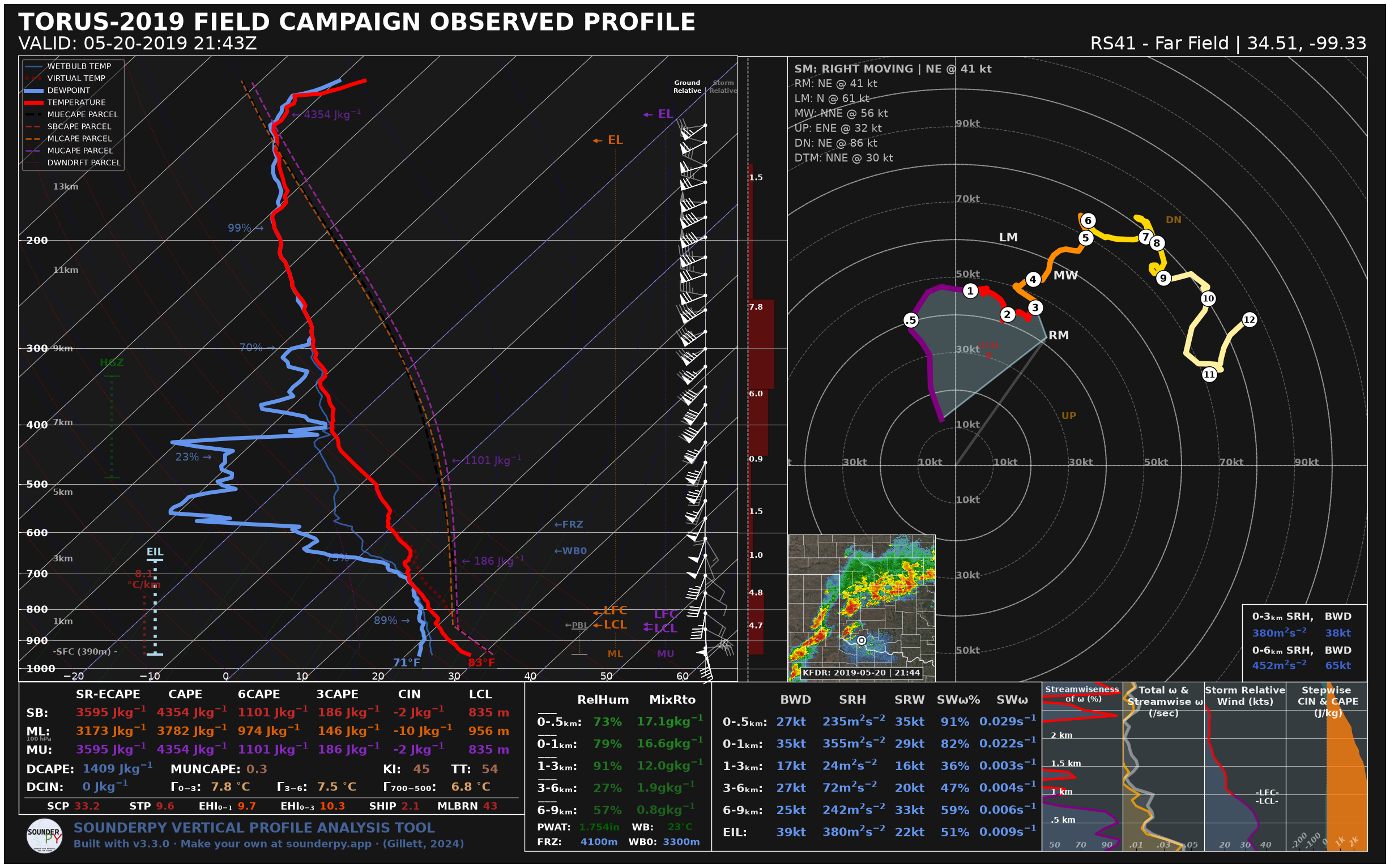
LETS PLOT THE DATA ON A SOUNDING AND HODOGRAPH
[5]:
# lets make a sounding!
# radar='single' shows the nearest NEXRAD site's reflectivity on the map.
# The default radar mosaic only keeps about the last month, so it can't cover this date.
spy.build_sounding(clean_data, dark_mode=True, color_blind=True, radar='single')
> SOUNDING PLOTTER FUNCTION
  ---------------------------------
    > PREPARING DATA
/home/kjgil/venvs/docsvenv/lib/python3.12/site-packages/numpy/lib/_function_base_impl.py:1687: UserWarning: Warning: converting a masked element to nan.
  return interp_func(x, xp, fp, left, right)
    > BUILDING SKEW-T LOG-P DIAGRAM
    > BUILDING HODOGRAPH
    > BUILDING MAP INSET
    > RADAR SCAN FOUND: Site: KFDR Scan: 2019-05-20 | 21:44z
Ignoring fixed x limits to fulfill fixed data aspect with adjustable data limits.
Ignoring fixed x limits to fulfill fixed data aspect with adjustable data limits.
Ignoring fixed y limits to fulfill fixed data aspect with adjustable data limits.
    > BUILDING ACCESSORY PLOTS
    > PLOTTING SOUNDING PARAMETERS
    > FIGURE LOADING...
    > COMPLETE --------
    > RUNTIME: 00:00:33
[ ]: