📈 Tools for Plotting Data
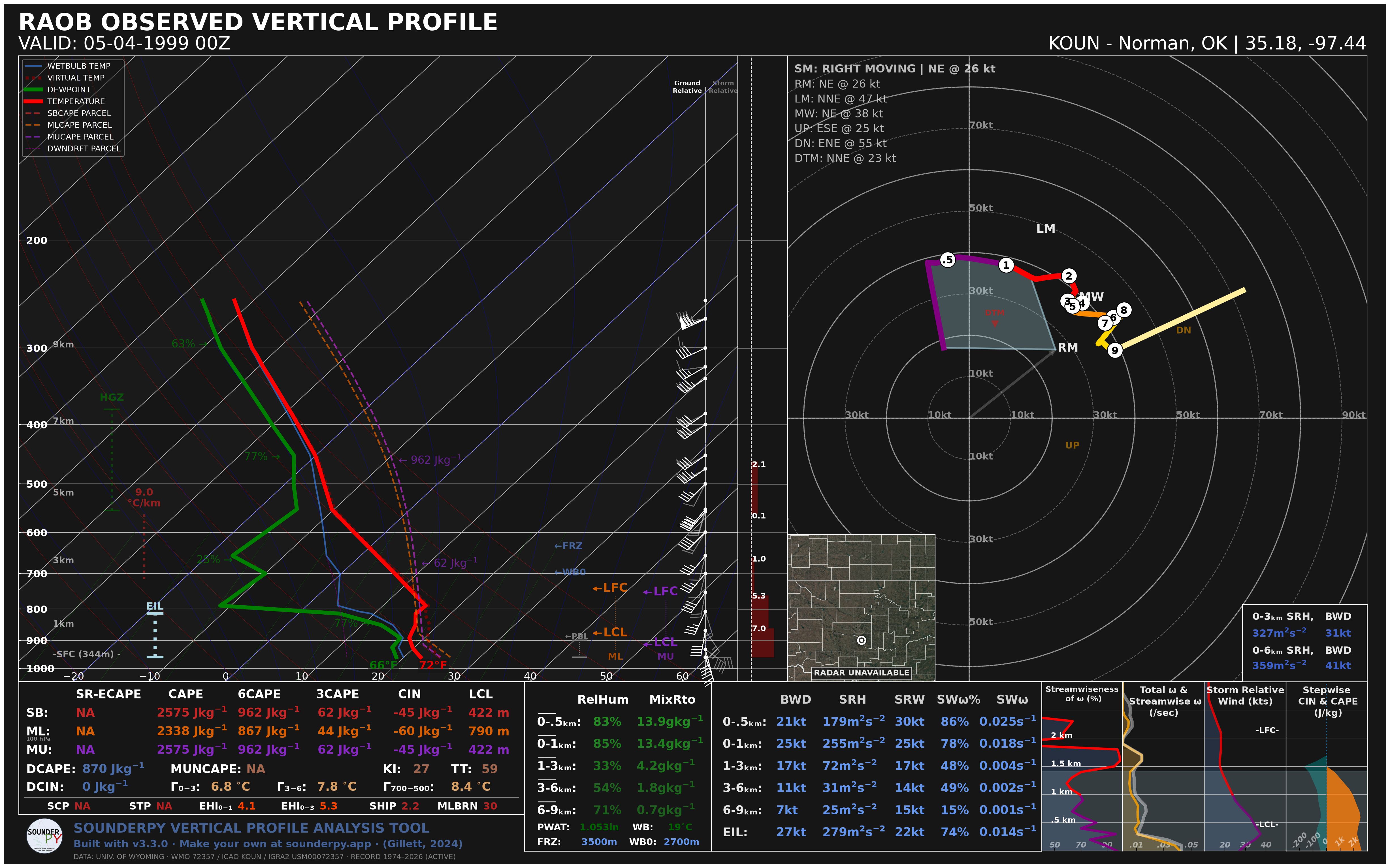
SounderPy can create general sounding and hodograph plots as well as composite sounding plots!
The full sounding plot that SounderPy creates is a complex figure with unique design geared towards severe convective storm environment analysis. As of v3.3.0, a long-overdue winter version of the full sounding figure is available.
These sounding plots are ‘my baby’ and I hope you find them useful! :)
Check out SounderPy’s 📊 Plot Gallery & example notebooks
Tip
Do your plots have funky scaling? This is a common issue for smaller screen sizes. To fix this, use the save=True kwarg in your plot function.
Building Soundings
While this function may appear complicated at first glance, there is actually only one required argument for this function (your sounding data: clean_data). The other arguments are simply optional settings for the plot!
- spy.build_sounding(
- clean_data,
- color_blind=False,
- dark_mode=False,
- storm_motion='right_moving',
- special_parcels=None,
- radar='mosaic',
- radar_time='sounding',
- map_zoom=2,
- modify_sfc=None,
- show_theta=False,
- hodo_boundary=None,
- dpi=100,
- save=False,
- filename='sounderpy_sounding',
- max_levels=250,
- ylim=None,
- theme=None,
- sr_hodo=False,
- mode='severe',
- show_obs=False,
Return a full sounding plot of SounderPy data,
plt- Parameters:
clean_data (dict, required) – the dictionary of data to be plotted (see 🌐 Tools for Getting Data)
color_blind (bool, optional, Default is
False) – whether or not to change the dewpoint trace line from green to blue for improved readability for color deficient users/readers.dark_mode (bool, optional, Default is
False.) –Truewill invert the color scheme for a ‘dark-mode’ sounding.storm_motion (str or list of floats, optional, Default is 'right_moving'.) – the storm motion used for plotting and calculations. Custom storm motions are accepted as a
listoffloatsrepresenting direction and speed. Ex:[270.0, 25.0]where ‘270.0’ is the direction in degrees and ‘25.0’ is the speed in kts. See the Storm Motion Logic section for more details.special_parcels (nested
listof twolists, optional, Default is None) – a nested list of special parcels from theecape_parcelslibrary. The nested list should be a list of two lists ([[a, b], [c, d]]) where the first list should include ‘highlight parcels’ and second list should include ‘background parcels’. For more details, see the Parcel Logic section. Another option is ‘simple’, which removes all advanced parcels making the plot quicker.radar (str,
"mosaic","single-site", orNone. Optional. Default ismosaic.) – whether to display mosaic reflectivity, single-site reflectivity, or no radar in the map inset.radar_time (str or
datetimeobj, optional, Default is"sounding".) – radar mosaic data valid time. May be"sounding"(uses the valid time of the sounding data),"now"(current time/date), or adatetimeobj Note: radar mosaic data only goes back 1 month from current datemap_zoom (int, optional, Default is
2.) – a ‘zoom’ level for the map inset as anint. Note: Settingmap_zoom=0will hide the mapmodify_sfc (None or dict, optional, default is None) – a
dictin the format{'T': 25, 'Td': 21, 'ws': 20, 'wd': 270}to modify the surface values of theclean_datadict. See the Surface Modification Logic section for more details.show_theta (bool, optional) – whether to replace the piecewise CAPE plot with theta & theta-e. Default is
Falsehodo_boundary (dict of lists, structured as
{'angle':[], 'color':[]}, optional, Default isNone) – plot a “boundary” (straight line) on the hodograph axis. Do so by providing an angle and a color. The angle represents the angle between zero-degrees (north) and the upper-half of the boundary line, to the right. Multiple boundaries can be plotted.dpi (int, optional, Default is 100.) – Dots per inch resolution of the figure.
save (bool, optional, Default is
False.) – whether to show the plot inline or save to a file.filename (str, optional, Default is
sounderpy_sounding.) – the filename by which a file should be saved to ifsave = True.max_levels (int or None, optional, Default is
250.) – the most vertical levels used to calculate and plot the sounding. Profiles with more levels are thinned to this many evenly spaced levels. Set toNoneto use every level.ylim (tuple of two numbers, optional, Default is
None, which shows the full profile.) – the skew-t’s pressure range as (bottom, top) in hPa, such as(1000, 700), to look at one part of the atmosphere. The temperature axis and pressure ticks fit to that range, while the rest of the figure still uses the full profile.theme (dict, optional, Default is
None.) – changes to the figure’s colors, such as{'border': 'k', 'temperature': 'navy', 'parcel': {'mu': 'black'}}. See Figure Colors for every setting.sr_hodo (bool, optional, Default is
False.) – draw the hodograph storm relative, shifting the winds by the storm motion fromstorm_motion. If the profile has no storm motion, the hodograph stays ground relative.mode (str,
"severe","winter", or"auto", optional, Default is"severe".) – which sounding to draw."severe"is the standard severe-weather sounding."winter"draws the winter sounding, built around precipitation type, snow growth, and winter hazards (see ❄️ Winter Soundings)."auto"draws the winter sounding when the surface wet-bulb temperature is below 35 degrees F, and the severe sounding otherwise. The winter sounding doesn’t usespecial_parcels,show_theta,sr_hodo, orhodo_boundary; if any are set, it warns and ignores them.show_obs (bool, optional, Default is
False.) – winter sounding only: draw a station model of the latest surface observation (METAR) near the profile, valid within an hour of the profile’s time, from the Iowa Environmental Mesonet. Needs internet access. Values missing from the report read “NA”.
- Returns:
plt, a SounderPy sounding figure.
- Return type:
plt
Examples
Severe sounding
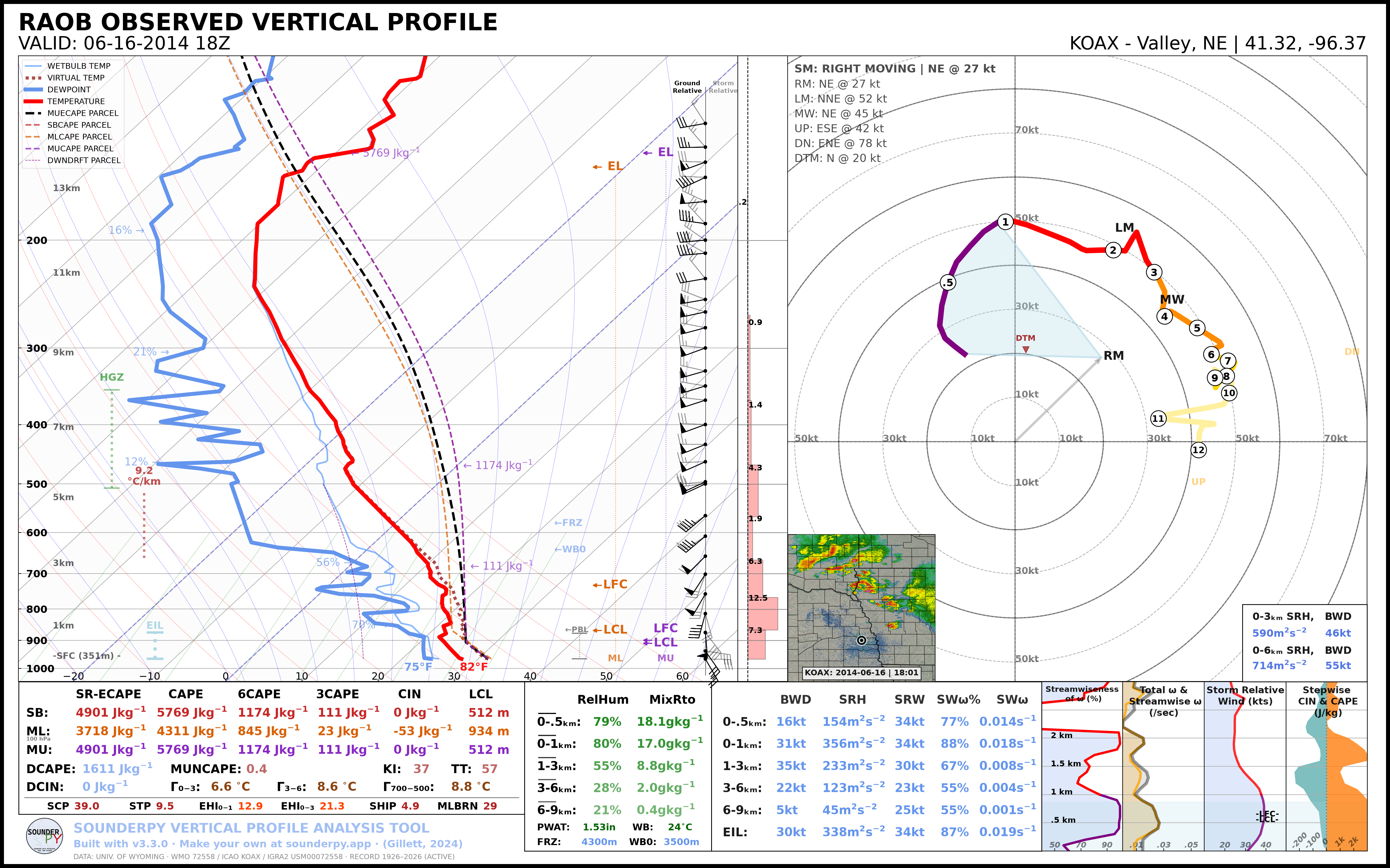
import sounderpy as spy

# get data | Note: any sounderpy data will work!
clean_data = spy.get_obs_data('OAX', '2014', '06', '16', '18')

# build the sounding!
spy.build_sounding(clean_data)
Winter sounding
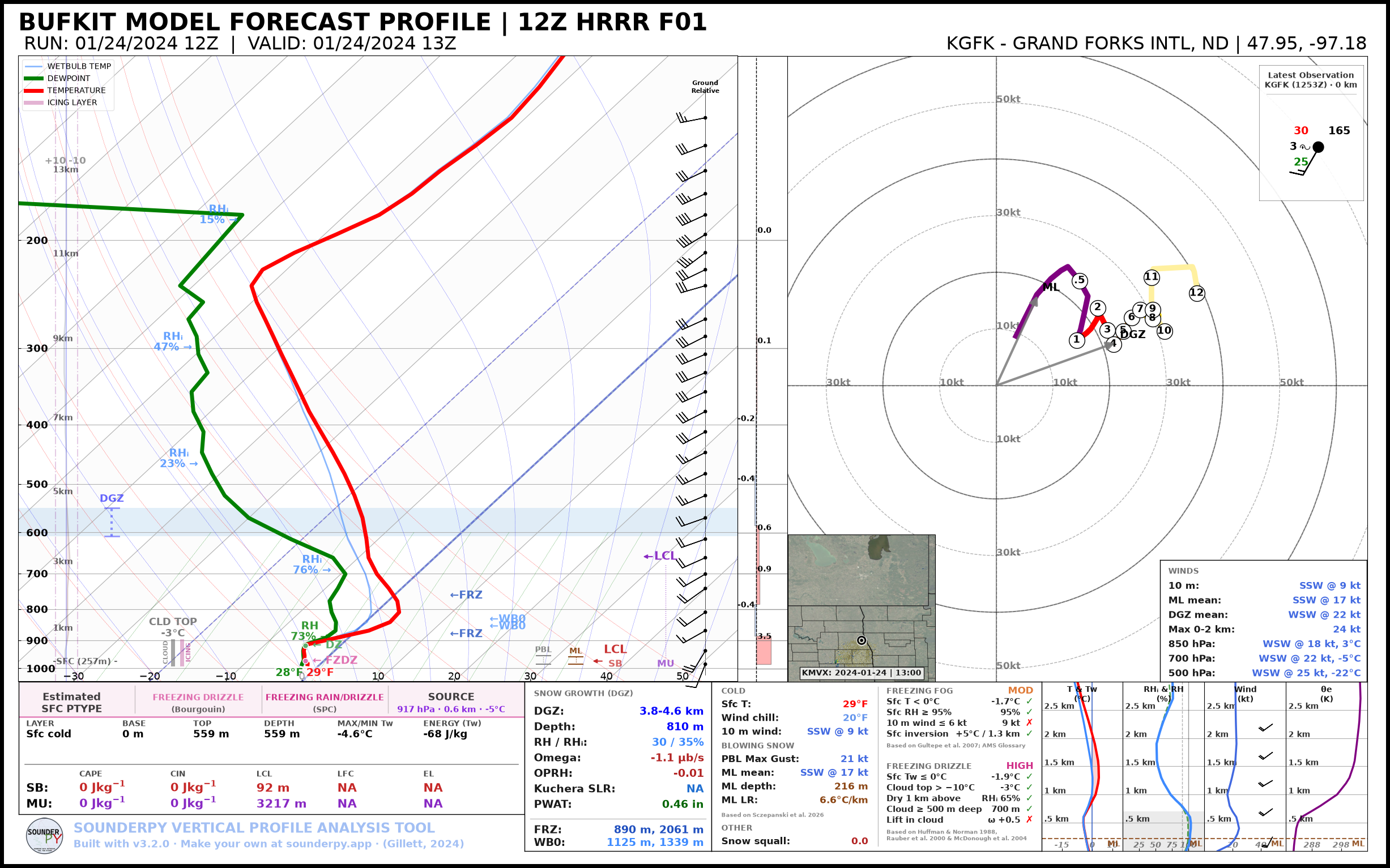
import sounderpy as spy

# get data | Note: any sounderpy data will work!
clean_data = spy.get_bufkit_data('hrrr', 'kgfk', 1,'2024', '01', '24', '12')

# build the winter sounding, with station plot and radar
spy.build_sounding(clean_data, mode='winter', show_obs=True, radar='single-site')
See ❄️ Winter Soundings for a guide to the winter sounding.
Building Hodographs
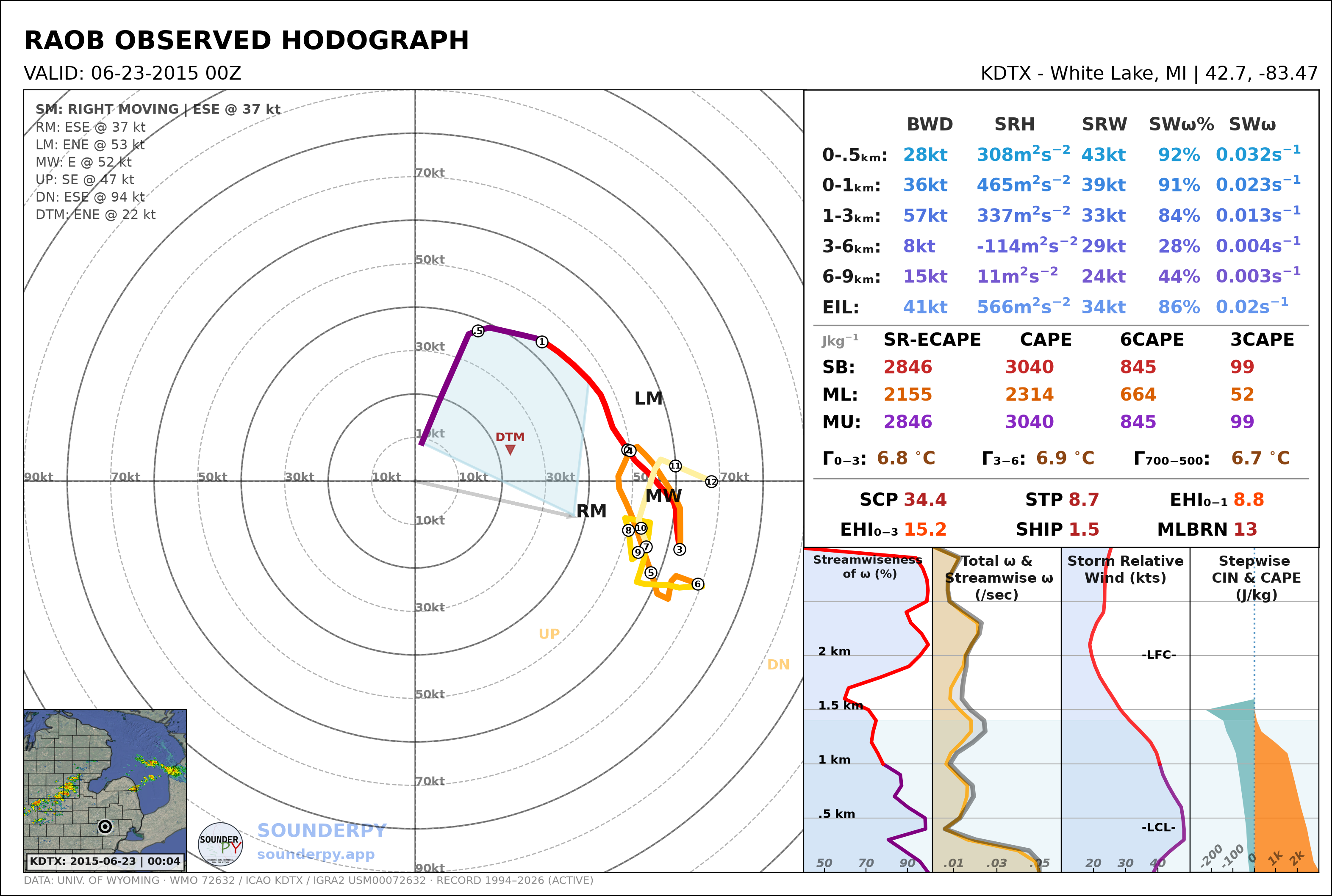
Very similarly to soundings, we can use the simple spy.build_hodograph() function:
- spy.build_hodograph(
- clean_data,
- dark_mode=False,
- storm_motion='right_moving',
- sr_hodo=False,
- modify_sfc=None,
- radar='mosaic',
- radar_time='sounding',
- map_zoom=2,
- hodo_boundary=None,
- dpi=100,
- save=False,
- filename='sounderpy_hodograph',
- max_levels=250,
- theme=None,
Return a full hodograph plot of SounderPy data,
plt- Parameters:
clean_data (dict, required) – the dictionary of data to be plotted (see 🌐 Tools for Getting Data)
dark_mode (bool, optional, Default is
False.) –Truewill invert the color scheme for a ‘dark-mode’ sounding.storm_motion (str or list of floats, optional, Default is 'right_moving'.) – the storm motion used for plotting and calculations. Custom storm motions are accepted as a
listoffloatsrepresenting direction and speed. Ex:[270.0, 25.0]where ‘270.0’ is the direction in degrees and ‘25.0’ is the speed in kts. See the Storm Motion Logic section for more details.sr_hodo (bool, optional, default is
False) – transform the hodograph from ground relative to storm relativemodify_sfc (None or dict, optional, default is None) – a
dictin the format{'T': 25, 'Td': 21, 'ws': 20, 'wd': 270}to modify the surface values of theclean_datadict.radar (str,
"mosaic","single-site", orNone. Optional. Default ismosaic.) – whether to display mosaic reflectivity, single-site reflectivity, or no radar in the map inset.radar_time (str or
datetimeobj, optional, Default is"sounding".) – radar mosaic data valid time. May be"sounding"(uses the valid time of the sounding data),"now"(current time/date), or adatetimeobj Note: radar mosaic data only goes back 1 month from current datemap_zoom (int, optional, Default is
2.) – a ‘zoom’ level for the map inset as anint. Note: Settingmap_zoom=0will hide the maphodo_boundary (dict of lists, structured as
{'angle':[], 'color':[]}, optional, Default isNone) – plot a “boundary” (straight line) on the hodograph axis. Do so by providing an angle and a color. The angle represents the angle between zero-degrees (north) and the upper-half of the boundary line, to the right. Multiple boundaries can be plotted.dpi (int, optional, Default is 100.) – Dots per inch resolution of the figure.
save (bool, optional, Default is
False.) – whether to show the plot inline or save to a file.filename (str, optional, Default is
sounderpy_hodograph.) – the filename by which a file should be saved to ifsave = True.max_levels (int or None, optional, Default is
250.) – the most vertical levels used to calculate and plot the hodograph. Profiles with more levels are thinned to this many evenly spaced levels. Set toNoneto use every level.theme (dict, optional, Default is
None.) – changes to the figure’s colors, such as{'border': 'k', 'temperature': 'navy', 'parcel': {'mu': 'black'}}. See Figure Colors for every setting.
- Returns:
plt, a SounderPy hodograph figure
- Return type:
plt
Example
import sounderpy as spy

# get data | Note: any sounderpy data will work!
clean_data = spy.get_obs_data('OAX', '2014', '06', '16', '18')

# build the hodograph!
spy.build_hodograph(clean_data, radar='single')
Building Composite Soundings
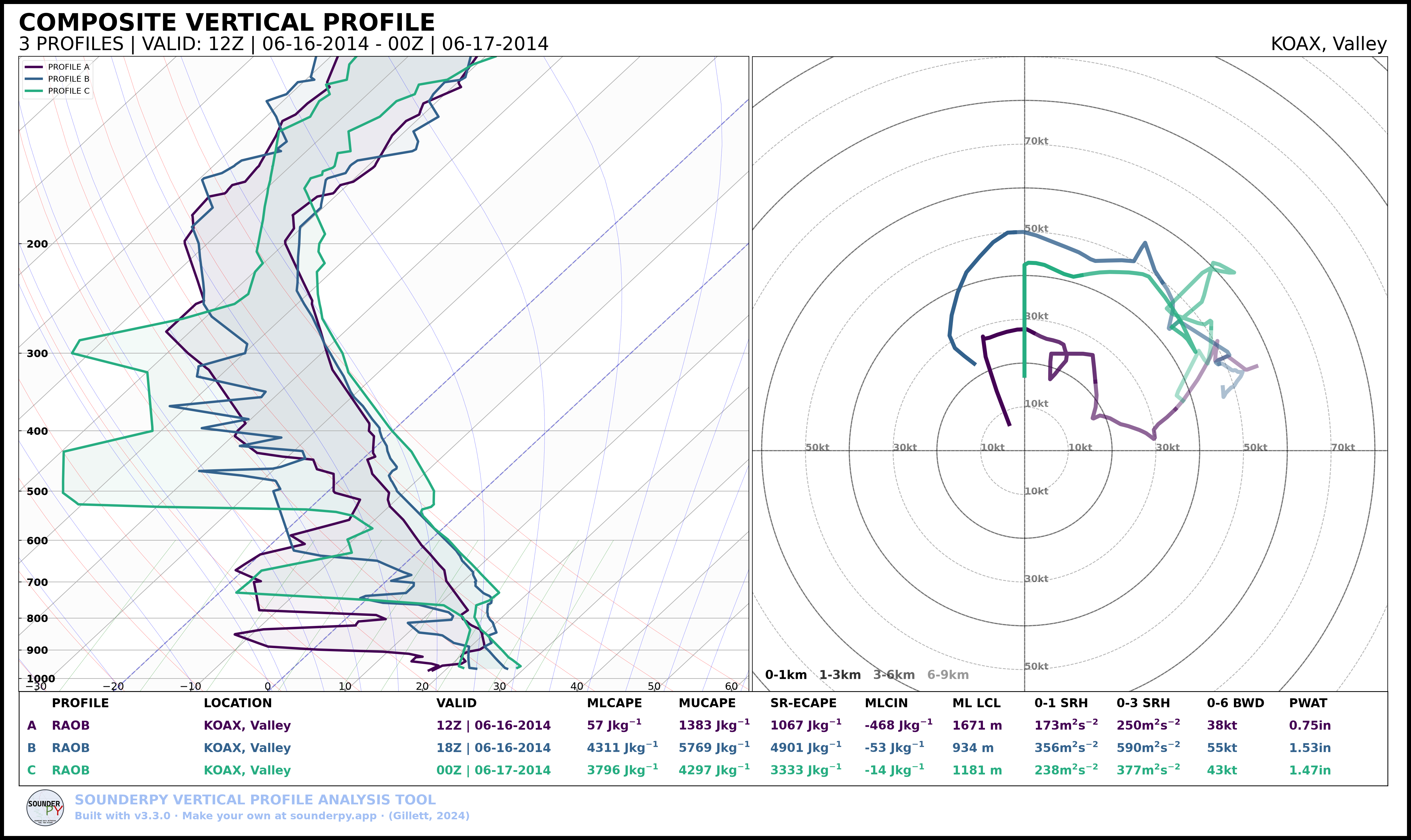
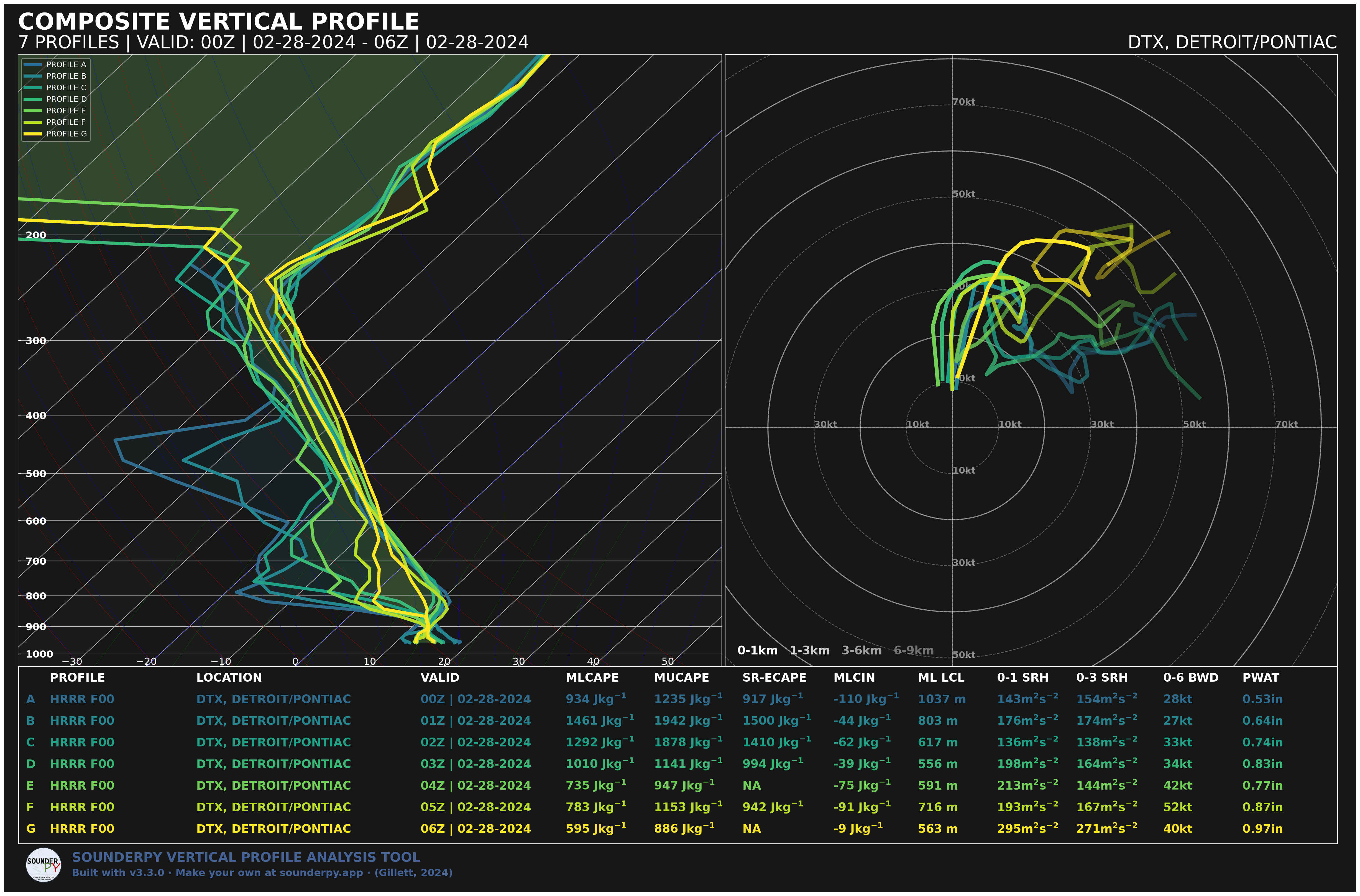
Sometimes we want to compare two or more profiles against each other. Perhaps at different locations or times, or we may want to compare different models or model run-times. SounderPy allows you to do this!
To do so, a list of ‘clean_data’ dicts is needed. If you want to customize the look of each profile, you can create equal length lists with alphas, linestyles, linewidths, & colors. See below:
- spy.build_composite(
- data_list,
- shade_between=True,
- cmap='viridis',
- colors=None,
- linestyles=None,
- alphas=None,
- linewidths=None,
- dark_mode=False,
- save=False,
- filename='sounderpy_composite',
- show_params=True,
- storm_motion='right_moving',
- max_levels=250,
- dpi=100,
- ylim=None,
- theme=None,
- style='full',
- sr_hodo=False,
Return a composite sounding plot of multiple profiles,
plt- Parameters:
data_list (list of dicts, required) – a list of
clean_datadictionaries for each profile to be plotted. Profiles may come from any mix of sources, such as observed, model, BUFKIT, ACARS, and custom data.shade_between (bool, optional, Default is
True.) – Lightly shade between the dewpoint & temperature trace. In many cases, this improves readability.cmap (
matplotlib.colors.LinearSegmentedColormaporstrrepresenting the name of a matplotlib cmap, optional, Default is ‘viridis’.) – a linear colormap, may be any custom or matplotlib cmap. The default uses only the part of ‘viridis’ that stands out from the figure’s background. Ifcolorskwarg is provided,colorswill be used instead.colors (list of strings, optional, Default is
None.) – A list of custom matplotlib color name strings. List length must match the number of profiles listed indata_list.alphas (list of floats, optional, Default is
None(sets alpha to 1)) – A list of custom alphas (0.0-1.0). List length must match the number of profiles listed indata_list.linestyles (list of strings, optional, Default is
None(sets linestyle to ‘-‘)) – A list of custom matplotlib linestyles. List length must match the number of profiles listed indata_list.linewidths (list of floats, optional, Default is
None(sets linewidth to 3).) – A list of custom linewidths. List length must match the number of profiles listed indata_list.dark_mode (bool, optional, Default is
False.) –Truewill invert the color scheme for a ‘dark-mode’ sounding.save (bool, optional, Default is
False) – whether to show the plot inline or save to a file.filename (str, optional, Default is
sounderpy_composite.) – the filename by which a file should be saved to ifsave = True.show_params (bool, optional, Default is
True.) – whether to compute each profile’s parameters and show them in the table. Setting this toFalseis faster.storm_motion (str or list of floats, optional, Default is 'right_moving'.) – the storm motion used to compute every profile’s parameters. See the Storm Motion Logic section for more details.
max_levels (int or None, optional, Default is
250.) – the most vertical levels used to calculate and plot each profile. Profiles with more levels are thinned to this many evenly spaced levels. Set toNoneto use every level.dpi (int, optional, Default is 100.) – Dots per inch resolution of the figure.
ylim (tuple of two numbers, optional, Default is
None, which shows the full profile.) – the skew-t’s pressure range as (bottom, top) in hPa, such as(1000, 700), to look at one part of the atmosphere. The temperature axis and pressure ticks fit to that range, while the rest of the figure still uses the full profile.theme (dict, optional, Default is
None.) – changes to the figure’s colors, such as{'border': 'k', 'temperature': 'navy', 'parcel': {'mu': 'black'}}. See Figure Colors for every setting.style (str, optional, Default is
'full'.) – the panels to show.'full'shows the skew-T and hodograph,'sounding'shows only the skew-T, and'hodograph'shows only the hodograph. Each style’s table lists the parameters that go with its panels.ylimis not used with'hodograph'.sr_hodo (bool, optional, Default is
False.) – draw the hodograph storm relative, shifting each profile’s winds by its own storm motion fromstorm_motion. Not used withstyle='sounding'. If any profile has no storm motion, the hodograph stays ground relative.
- Returns:
plt, a SounderPy composite sounding figure
- Return type:
plt
Note
colors, linestyles, alphas, and linewidths replace the older colors_to_use, ls_to_use, alphas_to_use, and lw_to_use. The old names still work for now, but show a FutureWarning and will be removed in a future release.
Examples
import sounderpy as spy

# get data | Note: any sounderpy data will work!
# this example looks at 3 profiles from OAX on Pilger-day.
clean_data1 = spy.get_obs_data('oax', '2014', '06', '16', '12')
clean_data2 = spy.get_obs_data('oax', '2014', '06', '16', '18')
clean_data3 = spy.get_obs_data('oax', '2014', '06', '17', '00')

# add each dict of data to a list
data_list = [clean_data1, clean_data2, clean_data3]

# build the composite!
spy.build_composite(data_list)
import sounderpy as spy

# get data | Note: any sounderpy data will work!

data_list = []
for hour in ['00', '01', '02', '03', '04', '05', '06']:
    cd = spy.get_bufkit_data('hrrr', 'dtx', 0, '2024', '02', '28', hour, hush=True)
    data_list.append(cd)

# and make it dark-mode for fun!
spy.build_composite(data_list, dark_mode=True, linewidths=[4 for cd in data_list])
Building VAD Hodographs
Caution
VAD hodograph support is experimental and may be more sensitive to missing, sparse, or unusual radar-derived wind profiles than the standard sounding hodograph workflow.
SounderPy now offers the ability to plot NEXRAD radar VAD data on a hodograph using the spy.build_vad_hodograph() function:
- spy.build_vad_hodograph(
- vad_data,
- save=False,
- dark_mode=False,
- storm_motion='right_moving',
- sr_hodo=False,
- filename='vad_hodograph',
- radar='mosaic',
- radar_time='sounding',
- map_zoom=2,
- hodo_boundary=None,
- dpi=100,
- theme=None,
Return a full hodograph plot of SounderPy VAD data,
plt- Parameters:
vad_data (dict, required) – the dictionary of VAD data to be plotted
dark_mode (bool, optional, Default is
False.) –Truewill invert the color scheme for a ‘dark-mode’ sounding.storm_motion (str or list of floats, optional, Default is 'right_moving'.) – the storm motion used for plotting and calculations. Custom storm motions are accepted as a
listoffloatsrepresenting direction and speed. Ex:[270.0, 25.0]where ‘270.0’ is the direction in degrees and ‘25.0’ is the speed in kts. See the Storm Motion Logic section for more details.sr_hodo (bool, optional, default is
False) – transform the hodograph from ground relative to storm relativesave (bool, optional, Default is
False) – whether to show the plot inline or save to a file.filename (str, optional, Default is
vad_hodograph.) – the filename by which a file should be saved to ifsave = True.radar (str,
"mosaic","single-site", orNone. Optional. Default ismosaic.) – whether to display mosaic reflectivity, single-site reflectivity, or no radar in the map inset.radar_time (str, optional, Default is
"sounding".) – the time of radar to show:"sounding"for the data’s valid time, or"now".map_zoom (int, optional, Default is
2.) – a ‘zoom’ level for the map inset as anint. Note: Settingmap_zoom=0will hide the maphodo_boundary (dict of lists, optional, Default is
None) – plot a “boundary” (straight line) on the hodograph axis, structured as{'angle':[], 'color':[]}.dpi (int, optional, Default is 100.) – Dots per inch resolution of the figure.
theme (dict, optional, Default is
None.) – changes to the figure’s colors, such as{'border': 'k', 'temperature': 'navy', 'parcel': {'mu': 'black'}}. See Figure Colors for every setting.
- Returns:
plt, a SounderPy sounding built with Matplotlib, MetPy, SharpPy, & SounderPy.
- Return type:
plt
Examples
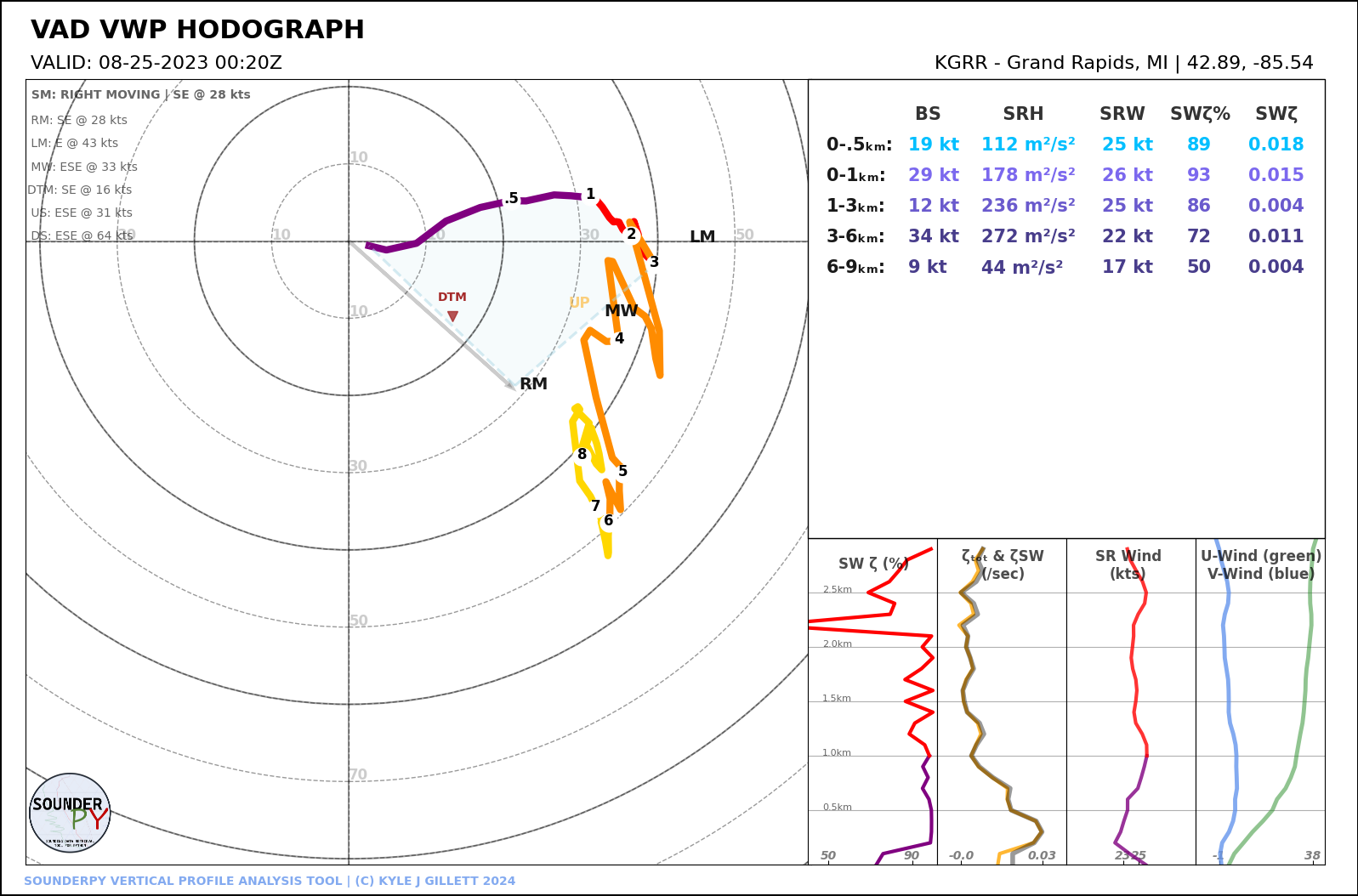
Figure Colors
Every plotting function accepts a theme dictionary that changes individual colors in the figure. Only the settings you include change; everything else keeps the light or dark color scheme. color_blind=True and dark_mode=True are applied first, so a theme can adjust them further.
spy.build_sounding(clean_data, theme={'border': 'k',
                                      'temperature': 'navy',
                                      'parcel': {'mu': 'black'}})
Parcel colors can be changed one at a time, as with 'parcel': {'mu': 'black'} above. An invalid setting name raises an error that lists every valid name.
Theme settings
Figure:
text,background,border,marker,barb,skew_line,shade_alphaSkew-T profiles:
temperature,dewpoint,virtual,wetbulbSkew-T background:
adiabat,isotherm,shadeParcels:
parcel(a dict withsb,ml, andmu),special_parcel,secondary_parcel,downdraftHodograph:
hodo_layers,height_marker,height_marker_edge,mcs,dtmSkew-T annotations:
pbl,eil,dgz,hgz,lapse_maxShared warm and cool values:
warm,cool,ascentTables:
moisture,moisture_strong,kinematics,kinematics_strong,kinematics_layers,ncape,lapse,composite_index,ehiAccessory panels:
bar_edge,pressure_line,low_fill,omega_zero,omega_reference,zero_line,streamwise,theta,u_wind,v_wind,cin,capeWatermark:
watermark
hodo_layers is a sequence of (bottom_m, top_m, color) layers, such as ((0, 1000, 'purple'), (1000, 3000, 'red')), and kinematics_layers is a sequence of five colors.
Watermark
SounderPy figures by default show the SounderPy logo and credit text. In a new addition, spy.set_watermark() allows you to change it for every figure made afterwards in the same Python session. This is especially useful for field campaign projects or university observations.
- spy.set_watermark(**settings)
Change the watermark on SounderPy figures, for this Python session. Pass only the settings to change. Calling this with no arguments restores the default watermark.
- Parameters:
show (bool, optional, Default is
True.) – whether to show the watermark text and logotitle (str, optional) – the top line of text, on every figure. By default, each figure uses its own text
subtitle (str, optional) – the bottom line of text, on every figure. By default, each figure uses its own text
logo (str or None, optional) – a path to an image to use as the logo, or
Nonefor no logo. By default, the SounderPy logo is usedcolor (str, optional) – the color of the text. By default, the figure’s
watermarktheme color is usedalpha (float, optional, Default is
0.6.) – the transparency of the text
Example
import sounderpy as spy

# use your own text and logo on every figure
spy.set_watermark(title='MY RESEARCH GROUP', subtitle='Made with SounderPy', logo='my_logo.png')

# hide the watermark
spy.set_watermark(show=False)

# restore the default watermark
spy.set_watermark()
Note
Watermark settings are shared by everything running in the same Python process.
Surface Modification Logic
Users may override the surface values of the clean_data dict, when creating a plot or returning sounding parameters, using the modify_sfc kwarg. This argument is a python dictionary. New to v3.3.0, the surface modification logic now includes three different “methods” of modification: “mix”, “blend”, and “replace”.
With the default 'method': 'mix', a surface temperature warmer than the profile is mixed upward along its dry adiabat until it meets the original profile, the depth a heated surface mixes to (Holzworth 1964). Through that layer, a new surface dewpoint is held at a constant mixing ratio, as in a well-mixed boundary layer. A cooler surface temperature, a dewpoint-only change, and wind changes will change only the surface level (i.e., no mixing). Dewpoint is never allowed to exceed temperature.
With 'method': 'blend', the temperature and dewpoint changes taper linearly from the surface to zero at depth meters above ground (500 m by default), so a warmer surface may give a superadiabatic layer of that depth while the profile above it is unchanged. For example, a surface 4°C warmer blended over 250 m adds 16 °C/km to that layer’s lapse rate. This option is usually unrealistic in the warm season, but may be useful in the cool season (e.g., blowing snow, lake effect, etc)
With 'method': 'replace', only the surface level changes, so a superadiabatic surface layer is kept. This suits cases where the lowest few hundred meters matter most.
The modify_sfc dict
T: Temperature, degrees CelsiusTd: Dewpoint, degrees Celsiusws: Wind speed, knotswd: Wind direction, meteorological degrees (north=0)method:'mix'(default),'replace', or'blend'depth: Depth of the blend, meters above ground ('blend'only, default 500 (meters))
Examples:
spy.build_sounding(clean_data, modify_sfc={'T':21, 'Td':19, 'ws': 30, 'wd':270})

spy.build_sounding(clean_data, modify_sfc={'T':21, 'Td':19})

spy.build_sounding(clean_data, modify_sfc={'ws': 30, 'wd':270})

spy.build_sounding(clean_data, modify_sfc={'T':-8, 'Td':-11, 'method':'replace'})

spy.build_sounding(clean_data, modify_sfc={'T':-8, 'Td':-11, 'method':'blend', 'depth':250})
Caution
Surface modification should be used carefully. Replacing the surface thermodynamic or wind state can materially alter parcel and kinematic calculations.
Storm Motion Logic
Users can define custom storm motions or choose from a number of ‘storm motion keys’ to change the storm motion considered by kinematic and thermodynamic parameters during calculations and plotting. All parameters that consider storm motion will be affected by the storm_motion kwarg.
Storm Motion Keys
"right_moving"— Bunkers right-moving supercell motion (default). Also"rm","right", or"right_mover""left_moving"— Bunkers left-moving supercell motion. Also"lm","left", or"left_mover""mean_wind"— 0-6km mean wind. Also"mw"or"mean"
Keys are not case sensitive. Any other value raises a ValueError.
Example:
storm_motion='left_moving'
Custom Storm Motions
Custom storm motions are supplied as:
[direction_degrees, speed_knots]
Direction follows the meteorological from convention. For example, 250 degrees at 45kts:
storm_motion = [250, 45]
Parcel Logic
SounderPy supports several parcel-ascent configurations, including pseudoadiabatic and irreversible-adiabatic ascent with entraining and non-entraining formulations. This toolkit comes from Amelia Urquhart’s ecape-parcels Python package, which is based on work by Peters et al. 2022.
When plotting soundings, users can choose from a number of parcel types to compute and plot, such as…
Pseudoadiabatic non-entraining ascent CAPE
Pseudoadiabatic entraining ascent CAPE
Irreversible Adiabatic non-entraining ascent CAPE
Irreversible Adiabatic entraining ascent CAPE
Each of these parcel types can be computed and plotted from a/the…
Surface-based parcel
Most-Unstable parcel
Mixed Layer parcel
How to use this feature
When plotting a full sounding using the build_sounding() function, use the kwarg special_parcels to choose which parcels you’d like to plot. This kwarg is a nested list ([[a, b], [c, d]]), where the first list contains ‘highlight’ parcels and the second list contains ‘background’ parcels. I.e., ‘highlighted’ parcels are darker and on top of ‘background’ parcels, which appear faded and behind the ‘highlight’ parcels.
Example:
special_parcels = [["sb_ia_ecape"], ["sb_ps_ecape", "sb_ps_cape"]]
By default, SounderPy will plot normal MU/ML/SB-CAPE parcels and an mu_ia_ecape parcel. You can override this by setting special_parcels to ‘simple’, which only plots the common MU/ML/SB-CAPE parcels. This can greatly reduce the plot-time!
Parcel Keys
Note the structure of the ‘parcel key’: sb_ia_ecape. This is broken into three components: ‘parcel-type’, ‘ascent-scheme’, and ‘entrainment-scheme’. You can make any parcel you like using this specific nomenclature: parcel-type_ascent-scheme_entrainment-scheme.
PARCEL-TYPES
sb: surface-based parcelmu: most-unstable parcelml: mixed-layer parcel
ASCENT-SCHEMES
ps: Pseudoadiabatic ascentia: Irreversible adiabatic ascent
ENTRAINMENT-SCHEMES
cape: non-entraining convective available potential energyecape: entraining convective available potential energy
Examples:
'sb_ia_ecape': surface-based irreversible adiabatic entraining CAPE'mu_ps_cape': most-unstable pseudoadiabatic CAPE'ml_ia_cape': mixed-layer irreversible adiabatic CAPE'sb_ps_ecape': surface-based pseudoadiabatic entraining CAPE
Setting special_parcels="simple" plots only the standard SB/ML/MU CAPE parcels and skips the additional MU ECAPE parcel, reducing calculation and plotting time.
Radar Logic
Knowing the location of a vertical profile relative to nearby meteorological phenomenon is vital in understanding what that vertical profile means for the atmosphere at a given time. To help with this, SounderPy employs the use of mapping & radar data to provide this information to a reader.
Using the Map
The map inset is controlled with map_zoom.
map_zoom=0disables the map.Larger positive values display a broader geographic area.
Using Radar
SounderPy offers two sources of radar data to the user. First is a CONUS reflectivity mosaic, and the other is single-site NEXRAD WSR-88D reflectivity. The CONUS mosaic is default because its fastest and easiest to plot, but data availability is only up to 30 days before the current date. Single-site radar goes back much further but data availability varies by site and date.
To plot radar on a sounding or hodograph, there are two kwargs to understand:
radar"mosaic": plots the CONUS reflectivity mosaic"single": plots single-site WSR-88D reflectivity closest to the latitude/longitude coordinates of the sounding.
radar_time"now": plots the most recent radar scan"sounding": plots the radar scan closest the time of the soundingdatetime(1999, 5, 4, 0, 27): or you may define your own time by providing a datetime obj. This will plot the nearest radar scan to the date/time provided.
About These Plots
SounderPy’s full sounding layout is designed to summarize thermodynamic and kinematic characteristics commonly examined in severe-convective-environment analysis.
The figure intentionally emphasizes physically interpretable profile quantities and parcel/kinematic diagnostics rather than displaying a large number of composite severe-weather indices.
The interpretation of any SounderPy figure depends on the source profile. Observed soundings, aircraft profiles, model forecasts, analyses, and reanalyses each have different sampling characteristics and limitations. Users should consider those limitations when interpreting calculated parameters and environmental diagnostics.
The data on these plots are considered, by most, to be useful in determining critical characteristics of the atmosphere related to supercellular storm mode and tornadogenesis.