
Plotting Soundings with BUFKIT Forecast Model Data
[1]:
# import sounderpy
import sounderpy as spy
Understanding SounderPy Functionality
To get model forecast data via BUFKIT, we need to use the get_bufkit_data() function
Reading the documentation on BUFKIT data access may prove useful before using this notebook: https://kylejgillett.github.io/sounderpy/reference/gettingdata.html#model-forecast-data-bufkit-profiles
[2]:
################################ THE FUNCTION ###################################
# to get bufkit data, we need to use the `get_bufkit_data()` function
# `get_bufkit_data(model, station, fcst_hour, run_year=None, run_month=None, run_day=None, run_hour=None)`
################################################################################


########################## TYPES OF BUFKIT DATA ################################
# we can access archived model forecasts from the GFS, NAM, NAMNEST, RAP, HRRR & RRFS
# or most recent run forecasts from the GFS, RAP, HRRR & RRFS
# (NCEP decommissioned the NAM & NAMNEST on November 2, 2026, so they are archive only;
# the SREF & HIRESW are discontinued and no longer available)
################################################################################


########################## WHERE DATA IS AVAILABLE #############################
# NOTE: bufkit forecast data is *only available at specific BUFKIT site locations*
# you can find them here: https://kylejgillett.github.io/sounderpy/reference/gettingdata.html#available-bufkit-sites
################################################################################


############################# LETS GET SOME DATA ###############################
# to get archived forecasts we need every kwarg. (a kwarg is a Keyword Argument, like 'year', and 'station')
# the line below will get us a 12z GFS forecast from 08/05/2023 at forecast hour 6 for bufkit site KMOP:

# clean_data = spy.get_bufkit_data('gfs', 'kmop', 6, '2023', '08', '05', '12')

# to get the most recent forecasts we use the same function, but we *don't need a year, month, day or hour kwarg!*
# you just need a model, station and forecast hour.
# this will get you the most recent HRRR run, at forecast hour 6, for
# site `KAMA` (AMARILLO ARPT(AWOS)):


clean_data = spy.get_bufkit_data('hrrr', 'kama', 6)
> BUFKIT DATA ACCESS FUNCTION
   ---------------------------------
    > COMPLETE --------
    > RUNTIME: 00:00:01
    > SUMMARY: SUMMARY: 15Z HRRR F06 for KAMA,AMARILLO ARPT(AWOS) at 11-11-2026-21Z

    > THERMODYNAMICS ---------------------------------------------
    --- SBCAPE: 0.0 | MUCAPE: 0.0 | MLCAPE: 0.0 | MUECAPE: --
    --- MU 0-3: 0.0 | MU 0-6: 0.0 | SB 0-3: 0.0 | SB 0-6: 0.0

    > KINEMATICS -------------------------------------------------
    --- 0-500 SRW: 14.6 knot | 0-500 SWV: 0.0 | 0-500 SHEAR: 1.3 | 0-500 SRH: -2.4
    --- 1-3km SRW: 18.4 knot | 1-3km SWV: 0.002 | 1-3km SHEAR: 12.9 | | 1-3km SRH: 26.6
    ==============================================================
[3]:
# Lets check out the BUFKIT data that we just accessed
# and stored in the `clean_data` variable:

# `clean_data` is a python dictionary of 'clean' vertical profile data
# it comes with temperature, dewpoint, pressure, height, u and v
# as well as a number of useful 'meta data'

clean_data
[3]:
{'p': Quantity(array([897.4, 894.8, 889.9, 881.5, 869.3, 853.6, 835.1, 815.1, 793.6,
        769.7, 743.6, 715.2, 684.5, 651.4, 616. , 578.1, 537.9, 498.5,
        462.6, 430.1, 400.3, 373. , 348. , 325.2, 304.4, 285.5, 268.2,
        252. , 237.2, 223.5, 209.6, 195.8, 181.9, 168. , 154.1, 140.2,
        126.3, 112.4,  98.6,  85.7,  75.3,  66.9,  59.1]), "hectopascal"),
 'z': Quantity(array([ 1107.56,  1132.41,  1179.36,  1260.26,  1378.7 ,  1532.87,
         1717.15,  1919.73,  2141.67,  2393.89,  2676.63,  2993.81,
         3348.84,  3747.56,  4194.64,  4698.35,  5262.02,  5846.25,
         6409.  ,  6946.69,  7466.91,  7970.72,  8458.54,  8927.69,
         9377.95,  9807.76, 10220.76, 10626.74, 11015.64, 11393.62,
        11798.85, 12227.68, 12691.21, 13191.61, 13735.12, 14327.97,
        14977.26, 15692.27, 16482.91, 17320.  , 18090.26, 18795.69,
        19537.4 ]), "meter"),
 'T': Quantity(array([ 19.04,  18.54,  18.04,  17.14,  15.94,  14.44,  12.64,  10.94,
          9.14,   7.44,   5.74,   4.04,   2.14,   0.84,  -0.66,  -3.76,
         -8.26, -13.36, -18.56, -23.46, -27.86, -31.16, -34.76, -38.56,
        -42.36, -45.86, -49.06, -52.06, -55.26, -56.96, -58.16, -57.96,
        -58.26, -57.96, -58.36, -59.46, -61.96, -65.36, -68.56, -69.86,
        -69.66, -69.16, -68.36]), "degree_Celsius"),
 'Td': Quantity(array([  -1.9 ,   -2.01,   -2.12,   -2.32,   -2.59,   -2.98,   -3.35,
          -7.09,   -9.55,  -14.51,  -17.56,  -18.87,  -19.38,  -24.38,
         -34.65,  -40.22,  -41.91,  -42.62,  -46.3 ,  -48.45,  -49.91,
         -48.93,  -46.99,  -47.6 ,  -48.76,  -49.92,  -52.53,  -56.79,
         -58.51,  -64.31,  -67.75,  -73.05,  -73.54,  -74.08, -100.49,
        -100.94, -101.43, -101.98, -102.58, -103.23, -103.82, -104.35,
        -104.91]), "degree_Celsius"),
 'u': Quantity(array([-5.2482574 , -5.83252942, -6.02452813, -6.22273633, -6.22273633,
        -6.22273633, -6.22223426, -6.41658839, -6.41257214, -7.00035713,
        -6.60539851, -5.05106103, -1.16658868,  6.02360592,  6.60644441,
         3.6942414 ,  1.55553072,  1.16483429,  2.72093627,  3.88886567,
         6.22193301, 16.90721667, 24.48758041, 27.21789607, 30.12480764,
        35.57102498, 40.43510884, 48.20396818, 53.06260488, 47.61891639,
        45.6744877 , 48.79206696, 46.07044968, 39.8503922 , 39.65123479,
        39.26642227, 37.71253735, 36.74029705, 36.35132035, 30.32005846,
        26.23777537, 25.07309584, 24.10116937]), "knot"),
 'v': Quantity(array([ -6.60979533,  -7.19230148,  -7.38416961,  -7.58377561,
         -7.58377561,  -7.58377561,  -7.38914073,  -7.19423335,
         -6.99564283,  -7.00035713,  -7.77230407,  -9.71541468,
        -10.6865135 ,  -8.35500878,  -5.82846397,  -8.36015433,
        -13.80262382, -17.4912567 , -13.99800364, -15.55112934,
        -15.16310158, -11.85615976, -13.41211414, -16.3283108 ,
        -15.7421747 , -14.3860725 , -13.0212278 , -11.07560615,
        -11.66657032, -17.49204683, -17.68845876, -20.02103398,
        -21.19003931, -25.84949209, -27.21080078, -27.98779166,
        -29.15807653, -29.93263558, -31.30019823, -27.59880532,
        -20.60263924, -16.32624467, -16.52095745]), "knot"),
 'omega': Quantity(array([-0.1, -0.1, -0.1, -0.1, -0.1, -0.1, -0.1, -0.2, -0.2, -0.3, -0.3,
        -0.2,  0. ,  0.1,  0.3,  0.3,  0.2,  0.1,  0. ,  0.1,  0.1,  0. ,
         0.1,  0.2,  0.2,  0.2,  0.1,  0. ,  0. , -0.1,  0. ,  0. , -0.1,
        -0.1,  0. ,  0. ,  0. ,  0.1,  0. ,  0. ,  0. ,  0. ,  0. ]), "pascal / second"),
 'site_info': {'site-id': 'KAMA',
  'site-name': 'AMARILLO ARPT(AWOS)',
  'site-lctn': 'UA',
  'site-latlon': [np.float64(35.23), np.float64(-101.7)],
  'site-elv': np.int64(1099),
  'source': 'BUFKIT FORECAST PROFILE',
  'model': 'HRRR',
  'fcst-hour': 'F06',
  'run-time': ['2026', '11', '11', '15'],
  'valid-time': ['2026', '11', '11', '21'],
  'data-source': 'PENN STATE BUFKIT'},
 'titles': {'top_title': 'BUFKIT MODEL FORECAST PROFILE | 15Z HRRR F06',
  'left_title': ' RUN: 11/11/2026 15Z  |  VALID: 11/11/2026 21Z',
  'right_title': 'KAMA - AMARILLO ARPT(AWOS), UA | 35.23, -101.7    '}}
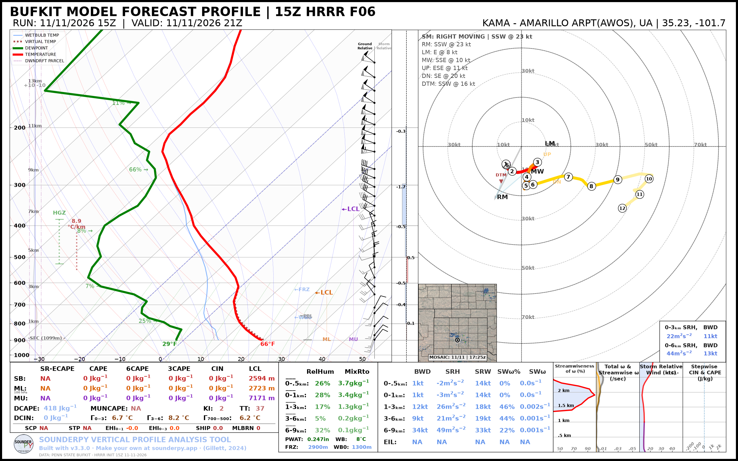
LETS PLOT THE DATA ON A SOUNDING AND HODOGRAPH
[4]:
# lets make a sounding!
spy.build_sounding(clean_data)
> SOUNDING PLOTTER FUNCTION
  ---------------------------------
    > PREPARING DATA
    > BUILDING SKEW-T LOG-P DIAGRAM
    > BUILDING HODOGRAPH
    > BUILDING MAP INSET
Ignoring fixed x limits to fulfill fixed data aspect with adjustable data limits.
Ignoring fixed x limits to fulfill fixed data aspect with adjustable data limits.
Ignoring fixed y limits to fulfill fixed data aspect with adjustable data limits.
    > BUILDING ACCESSORY PLOTS
    > PLOTTING SOUNDING PARAMETERS
    > FIGURE LOADING...
    > COMPLETE --------
    > RUNTIME: 00:00:04
[ ]: