
❄️ Winter Soundings
SounderPy’s winter sounding keeps the layout of the full sounding, but fills each part with winter content: precipitation type and how falling precipitation changes phase on its way down, melting and refreezing layers, clouds and icing, snow growth, and winter hazards.
This tutorial covers:
making a winter sounding from BUFKIT, RAOB, and ACARS data;
letting SounderPy choose between the severe and winter soundings;
adding the latest surface observation;
which plot options the winter sounding uses;
a guided tour of every part of the figure.
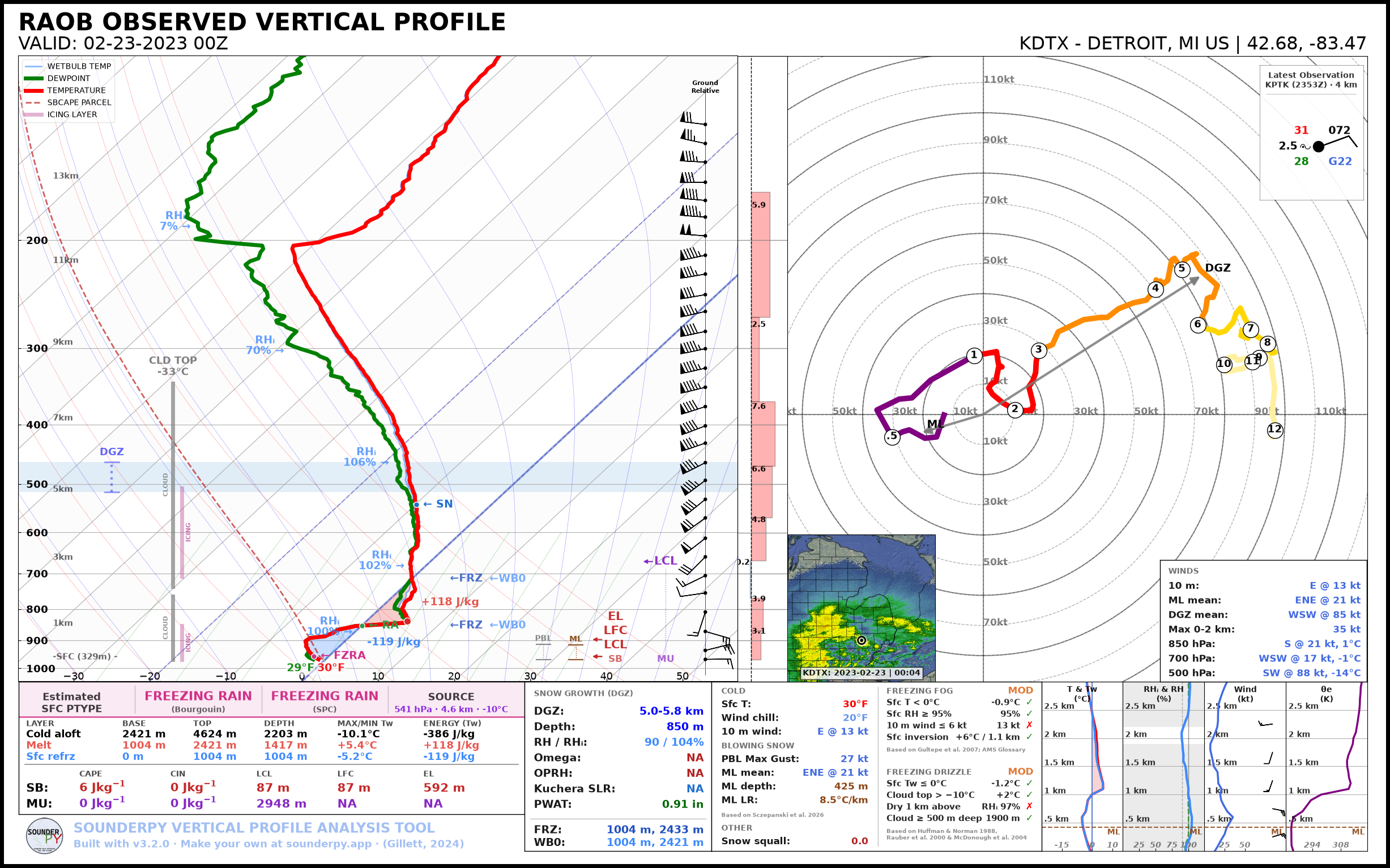
The Detroit, MI RAOB at 00 UTC on 23 February 2023, during an ice storm.
Make a Winter Sounding
Any SounderPy data works. Pass mode='winter' to build_sounding():
BUFKIT forecast
import sounderpy as spy

clean_data = spy.get_bufkit_data('hrrr', 'kgfk', 1, '2024', '01', '24', '12')

spy.build_sounding(clean_data, mode='winter')
Observed sounding (RAOB)
clean_data = spy.get_obs_data('DTX', '2023', '02', '23', '00')

spy.build_sounding(clean_data, mode='winter', radar='single-site')
ACARS aircraft profile
clean_data = spy.acars_data('2024', '01', '15', '14').get_profile('DEN_1420')

spy.build_sounding(clean_data, mode='winter')
Note
RAOB and ACARS profiles have no omega (vertical motion), so the omega-based values on the figure read “NA”.
Let SounderPy Choose
With mode='auto', SounderPy draws the winter sounding when the surface
wet-bulb temperature is below 35 degrees F, and the severe sounding otherwise:
spy.build_sounding(clean_data, mode='auto')
The surface wet-bulb temperature and the chosen sounding are printed while the figure builds.
Add the Latest Surface Observation
show_obs=True draws a station model of the latest surface observation
(METAR) from the station nearest the profile, valid within an hour of the
profile’s time. The observation comes from the Iowa Environmental Mesonet, so
this needs internet access:
spy.build_sounding(clean_data, mode='winter', show_obs=True)
The station model sits in the upper-right corner of the hodograph, with the station, the observation time, and its distance from the profile above it. Values missing from the report (such as a temperature from a station that only reports wind and visibility) read “NA”. If no observation is found, the figure is drawn without one.
Plot Options
The winter sounding uses the same color_blind, dark_mode,
storm_motion, radar, radar_time, map_zoom, modify_sfc,
dpi, save, filename, max_levels, ylim, and theme
options as the severe sounding. Its radar inset shows reflectivity from -30 to
65 dBZ, so light snow shows up.
It doesn’t use special_parcels, show_theta, sr_hodo, or
hodo_boundary. If any are set, SounderPy warns and ignores them.
A Tour of the Figure
The images below come from the Detroit ice storm sounding above.
The Skew-T
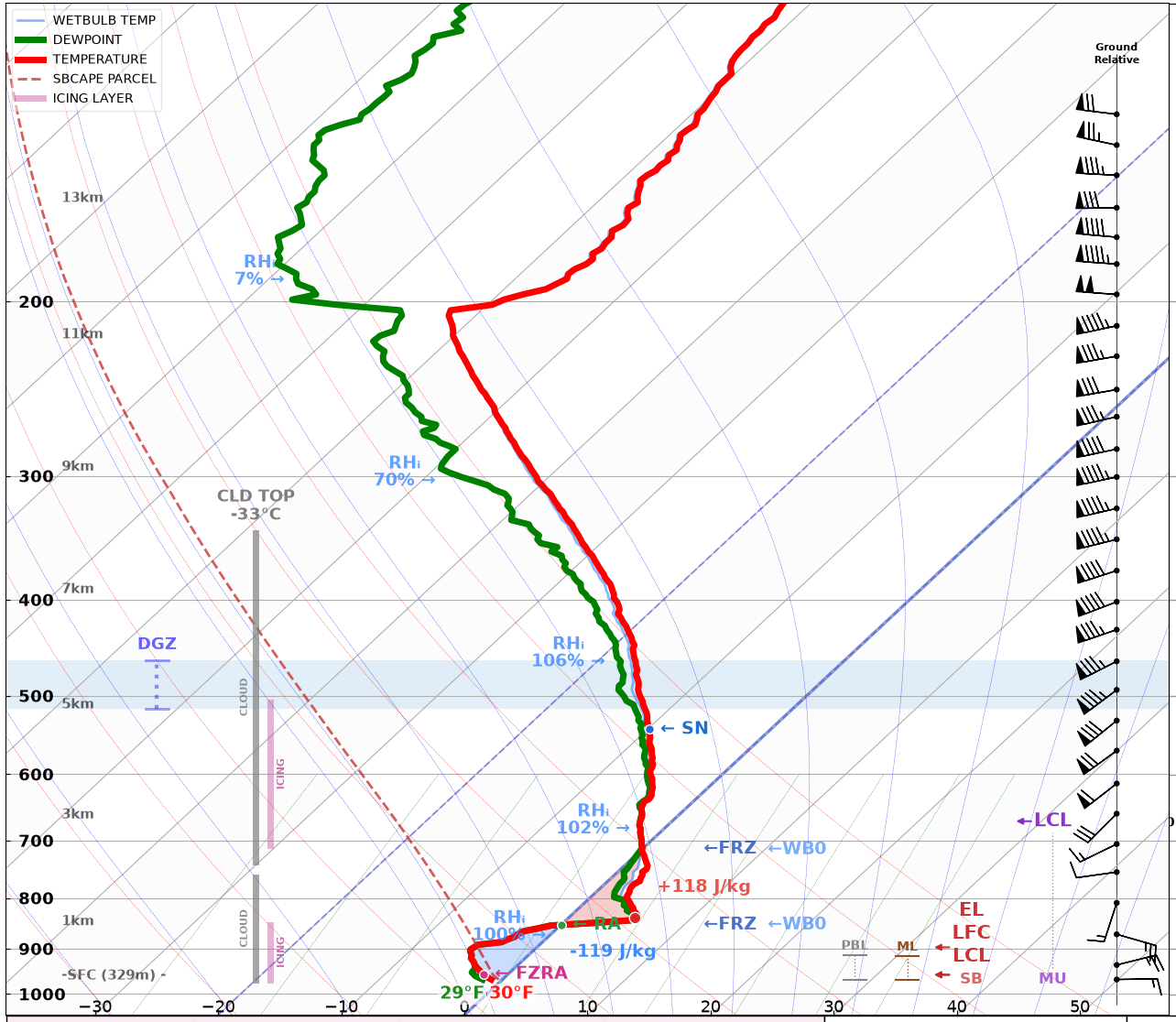
The skew-T shows the temperature, dewpoint, and wet-bulb temperature, plus:
Precipitation phase: labels on the temperature trace mark the phase of falling precipitation at its source and wherever it changes on the way down, such as
SNtoRAin a warm layer, thenFZRAat the surface. Snow carries its snow-to-liquid ratio (such asSN 22:1).Melting and refreezing layers: red shading where the wet-bulb temperature is above 0 °C (melting) and blue shading where it is below 0 °C under a warm layer (refreezing), each labeled with its energy in J/kg.
Freezing levels:
←FRZmarks every height where the temperature crosses 0 °C, and←WB0where the wet-bulb temperature does. The warm nose, the warmest point of a warm layer aloft, is marked with a dot.RH labels: RH over ice (RHᵢ) below 0 °C and over water above it, at 1, 3, 6, 9, and 12 km.
Bars on the left: the dendritic growth zone (DGZ, also shaded across the skew-T), cloud layers (with the temperature at the top of the highest one), and icing layers.
Bars on the right: the PBL (SHARPpy’s), and the surface-based (SB) and most-unstable (MU) parcels’ LCL, LFC, and EL.
Between the skew-T and the hodograph are temperature advection and, for data with it, omega.
Precipitation Type and Layers
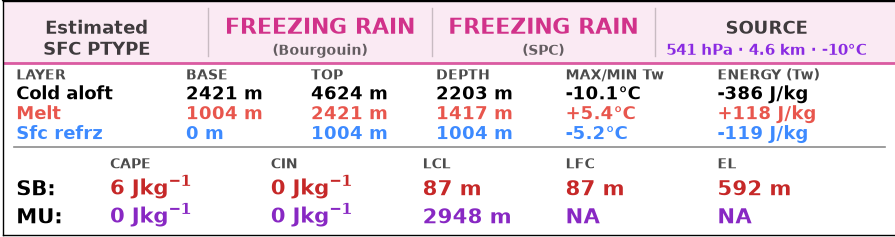
The band across the top gives the estimated surface precipitation type from two methods: Bourgouin’s energy method, computed from the wet-bulb temperature as in the revised method of Birk et al. (2021) and labeled “Bourgouin/Birk”, and SHARPpy’s best guess (from the SPC), followed by the precipitation source: the pressure, height, and temperature of the level the precipitation falls from.
The Bourgouin/Birk type follows the precipitation down, layer by layer, using the melting energy (ME) of each warm layer and the refreezing energy (RE) of each cold layer:
Warm layer at the surface (Bourgouin 2000): snow or sleet stays frozen below 5.6 J/kg, partly melts from 5.6 to 13.2 J/kg, and melts completely above that.
Warm layer aloft (Birk et al. 2021): it stays frozen below 9.4 J/kg, partly melts from 9.4 to 15 J/kg, and melts completely above that. These are where Birk et al.’s chance of snow, 1540 e-0.29 ME, is 100 % and 20 %.
Cold layer below a warm layer aloft (Birk et al. 2021): partly melted precipitation refreezes to sleet. Fully melted drops refreeze to sleet when RE is above 208 + 0.08 ME, give a freezing rain and sleet mix from 117 + 0.08 ME, and otherwise stay liquid.
Birk et al. (2021) built their thresholds from freezing rain, sleet, and mixed cases, so Bourgouin’s (2000) are kept for rain or snow under a warm surface layer. Birk et al. apply theirs to column totals; here they are applied to each layer in turn.
Below it, the layer table lists each layer between the source and the surface, top first: its base, top, depth, warmest or coldest wet-bulb temperature, and melting (positive) or refreezing (negative) energy. Under the table are the SB and MU parcels’ CAPE, CIN, LCL, LFC, and EL.
Snow Growth
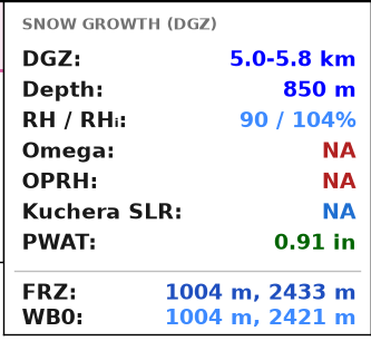
The snow growth box describes the dendritic growth zone (-12 to -17 °C) that makes the snow. When the profile has more than one layer in that range, it’s the one with the most cloud in it. The box gives:
the DGZ’s height, depth, mean RH and RHᵢ, and mean omega;
OPRH (omega x PWAT x RH in the DGZ), a measure of snow production;
the Kuchera snow-to-liquid ratio, when snow reaches the surface;
PWAT;
every height where the temperature (FRZ) and the wet-bulb temperature (WB0) cross 0 °C.
Winter Hazards
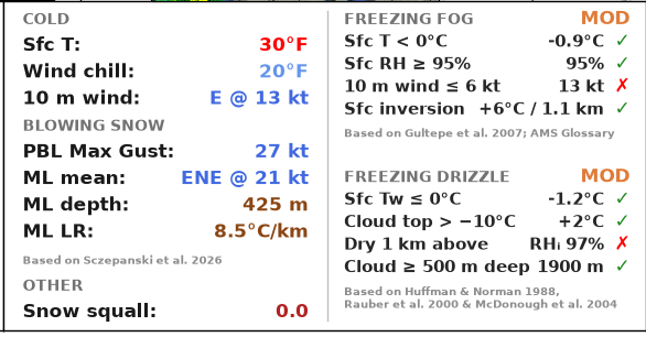
The left column gives:
Cold: surface temperature, wind chill, and the 10 m wind;
Blowing snow: the PBL gust (the strongest wind between the surface and the PBL top, which mixing could bring down), and the PBL mean wind, depth, and lapse rate;
Other: the snow squall parameter.
The right column checks the ingredients for freezing fog and for freezing drizzle. Each ingredient shows its value and whether it is met (✓ or ✗), and the section title gives a potential level from the ingredients met: NONE, LOW, MOD, or HIGH. These are ingredient checks, not forecasts.
Hodograph, Winds, and Surface Observation
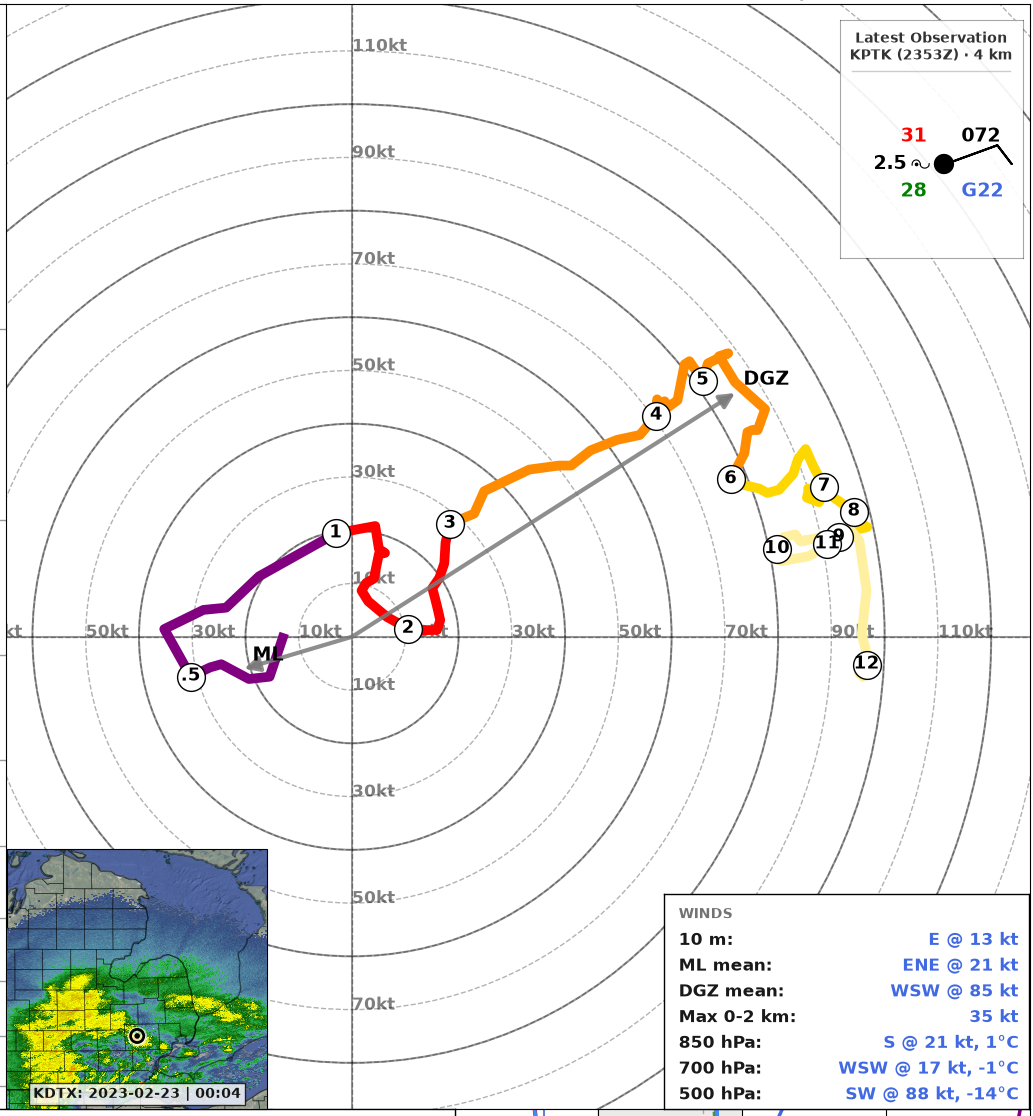
The hodograph shows the winds from the surface to 12 km, with arrows for the PBL and DGZ mean winds: the flow that blowing snow and lake-effect bands follow, and the flow where snow grows. The winds box in the lower-right corner lists the 10 m wind, the PBL and DGZ mean winds, the 0-2 km max wind, and the wind and temperature at 850, 700, and 500 hPa.
With show_obs=True, the station model of the latest surface observation is
in the upper-right corner: temperature (top left) and dewpoint (bottom left) in
degrees F, visibility in miles and present weather (left), coded sea-level
pressure (top right), gust (bottom right), sky cover in the circle, and the
wind barb.
Side Panels
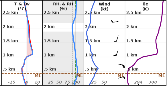
Four panels show the lowest 3 km:
T & Tw: temperature and wet-bulb temperature, with melting shaded;
RHᵢ & RH: RH over ice (solid) and over water (dashed), with clouds shaded;
Wind: wind speed (line) and direction (barbs);
θe: equivalent potential temperature.
The DGZ is shaded on each panel when it is in the lowest 3 km, and a dashed line marks the top of the PBL.
Winter Values in Code
The values on the figure are available as a dictionary with
spy.winter_params(), which returns every sounding_params value plus a
winter dictionary:
params = spy.winter_params(clean_data).calc()

params['winter']['ptype']
params['winter']['dgz_depth']
See 🛠️ Helper Tools for details.
References
The methods and thresholds behind the winter sounding come from these sources. A few thresholds are SounderPy’s own choices: RHᵢ of at least 90 % for cloud, 0 to -15 °C for icing, 95 % and 6 kt for freezing fog, and the 2 km cloud base, 75 % RHᵢ, and 500 m depth for freezing drizzle.
Alduchov, O. A., and R. E. Eskridge, 1996: Improved Magnus form approximation of saturation vapor pressure. J. Appl. Meteor., 35, 601-609, https://doi.org/10.1175/1520-0450(1996)035<0601:IMFAOS>2.0.CO;2. (RH over ice)
Banacos, P. C., A. N. Loconto, and G. A. DeVoir, 2014: Snow squalls: Forecasting and hazard mitigation. J. Operational Meteor., 2 (12), 130-151, https://doi.org/10.15191/nwajom.2014.0212. (snow squall parameter)
Bernstein, B. C., and Coauthors, 2005: Current icing potential: Algorithm description and comparison with aircraft observations. J. Appl. Meteor., 44, 969-986, https://doi.org/10.1175/JAM2246.1. (icing layers)
Birk, K., E. Lenning, K. Donofrio, and M. T. Friedlein, 2021: A revised Bourgouin precipitation-type algorithm. Wea. Forecasting, 36, 425-438, https://doi.org/10.1175/WAF-D-20-0118.1. (wet-bulb energies; thresholds for warm layers aloft)
Blumberg, W. G., K. T. Halbert, T. A. Supinie, P. T. Marsh, R. L. Thompson, and J. A. Hart, 2017: SHARPpy: An open-source sounding analysis toolkit for the atmospheric sciences. Bull. Amer. Meteor. Soc., 98, 1625-1636, https://doi.org/10.1175/BAMS-D-15-00309.1. (SPC precipitation type, OPRH)
Bourgouin, P., 2000: A method to determine precipitation types. Wea. Forecasting, 15, 583-592, https://doi.org/10.1175/1520-0434(2000)015<0583:AMTDPT>2.0.CO;2. (precipitation type: warm surface layer)
Gultepe, I., and Coauthors, 2007: Fog research: A review of past achievements and future perspectives. Pure Appl. Geophys., 164, 1121-1159, https://doi.org/10.1007/s00024-007-0211-x. (freezing fog)
Holzworth, G. C., 1964: Estimates of mean maximum mixing depths in the contiguous United States. Mon. Wea. Rev., 92, 235-242, https://doi.org/10.1175/1520-0493(1964)092<0235:EOMMMD>2.3.CO;2. (PBL depth)
Huffman, G. J., and G. A. Norman Jr., 1988: The supercooled warm rain process and the specification of freezing precipitation. Mon. Wea. Rev., 116, 2172-2182, https://doi.org/10.1175/1520-0493(1988)116<2172:TSWRPA>2.0.CO;2. (precipitation source phase, freezing drizzle)
Libbrecht, K. G., 2005: The physics of snow crystals. Rep. Prog. Phys., 68, 855-895, https://doi.org/10.1088/0034-4885/68/4/R03. (DGZ)
McDonough, F., B. C. Bernstein, M. K. Politovich, and C. A. Wolff, 2004: The Forecast Icing Potential (FIP) algorithm. Preprints, 11th Conf. on Aviation, Range, and Aerospace Meteorology, Hyannis, MA, Amer. Meteor. Soc., 3.2. (icing layers, freezing drizzle)
NOAA VLab: NWP snow accumulation products. Forecast Guide. (Kuchera snow-to-liquid ratio, developed by E. Kuchera, Air Force Weather Agency)
NWS, 2001: Wind chill chart. https://www.weather.gov/safety/cold-wind-chill-chart. (wind chill)
Osczevski, R., and M. Bluestein, 2005: The new wind chill equivalent temperature chart. Bull. Amer. Meteor. Soc., 86, 1453-1458, https://doi.org/10.1175/BAMS-86-10-1453. (wind chill)
Rauber, R. M., L. S. Olthoff, M. K. Ramamurthy, and K. E. Kunkel, 2000: The relative importance of warm rain and melting processes in freezing precipitation events. J. Appl. Meteor., 39, 1185-1195, https://doi.org/10.1175/1520-0450(2000)039<1185:TRIOWR>2.0.CO;2. (precipitation source phase, freezing drizzle)
Takahashi, T., T. Endoh, G. Wakahama, and N. Fukuta, 1991: Vapor diffusional growth of free-falling snow crystals between -3 and -23 °C. J. Meteor. Soc. Japan, 69, 15-30, https://doi.org/10.2151/jmsj1965.69.1_15. (DGZ)